Sort and filter data in Excel without scrambling your rows
Click one cell in the column (don't select just that column) and use Data › Sort & Filter › Sort A to Z or Sort Z to A. For several criteria, use Data › Sort › Add Level. To filter, click Data › Filter (Ctrl+Shift+L) and use the arrows on the headers. To total only the visible rows, use =SUBTOTAL(9,D2:D9).
Maybe it's happened to you: you sort the amount column from largest to smallest and suddenly every amount sits next to the wrong customer. Or you filter one region, add it up and get the total for all of them. Sort and filter look like simple buttons, but one click in the wrong place can ruin a whole list.
Think of each row as an index card: date, customer, region and amount are stapled together. Sorting changes the order of the cards; filtering sets aside the ones you don't need for now, without throwing them away. The danger comes when you pull a column away from its staples.
In this guide you'll sort by one and by several criteria without breaking rows, filter by text and by amount, and calculate totals that respect the filter.
What you'll learn
- How to sort by one column without mixing up each row's data
- How to sort by several criteria at once (region, then amount)
- How to filter by values, by text and by number conditions
- How to total only the visible rows with
=SUBTOTAL(9,D2:D9) - How to clear filters and see everything again
Step by step
Prepare the list: headers on top and no empty rows
Excel sorts and filters the data region around your cursor: the block of cells surrounded by empty rows and columns. That's why you need a header row and no empty rows in the middle; if there is one, Excel will only sort the part above or below it.
In the example you have one week of sales in A1:D9: Date, Customer, Region and Amount.
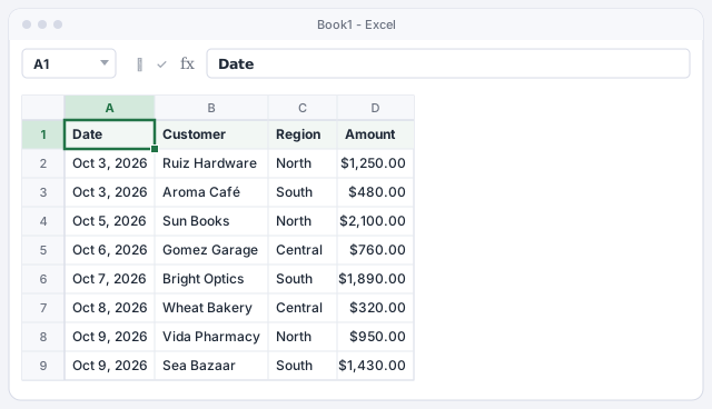
If you turn the list into a table (Insert › Table), Excel always knows where it starts and ends, and the filters come built in.
Sort by one column with a single click
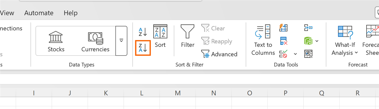
Click a single cell in the Amount column (for example, D2). Go to Data › Sort & Filter and click Sort Z to A (the ZA button with an arrow). Excel sorts from largest to smallest and moves each whole row: Sun Books rises to the top with its $2,100.00, its date and its region.
Sort A to Z (AZ) sorts smallest to largest, A to Z, or oldest to newest date. The same buttons are under Home › Editing › Sort & Filter.
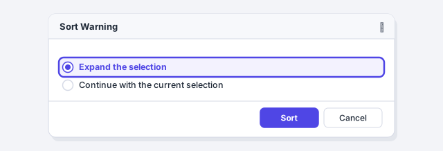
If you see “Sort Warning”, choose “Expand the selection”
This is the mistake that scrambles rows. If you select the entire column (click the letter D) before sorting, Excel asks what to do with the neighboring columns. Always choose Expand the selection and click Sort.
If you choose Continue with the current selection, Excel sorts only the amounts and leaves dates and customers where they were: every amount ends up on another customer's row.
If you've already sorted wrongly, press Ctrl+Z immediately. Once the file is saved and closed, there's no way to get the original order back.
Sort by several criteria with Data › Sort
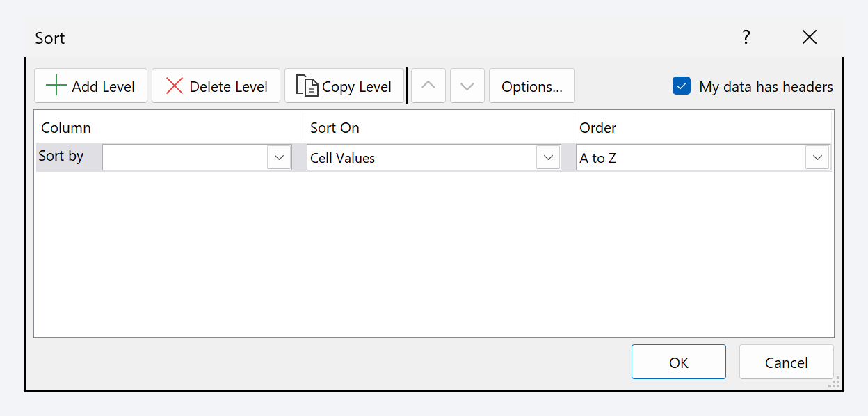
To see sales grouped by region and, within each region, from largest to smallest amount, go to Data › Sort & Filter › Sort. Make sure My data has headers is checked.
- Under Sort by, choose Region, Cell Values, A to Z.
- Click Add Level. Under Then by, choose Amount, Cell Values, Largest to Smallest.
- Click OK.
Result: first Central (Gomez Garage, Wheat Bakery), then North (Sun Books, Ruiz Hardware, Vida Pharmacy) and finally South (Bright Optics, Sea Bazaar, Aroma Café).
Turn on filters
With a cell in the list selected, go to Data › Sort & Filter › Filter, or press Ctrl+Shift+L. An arrow appears on each header. Filtering doesn't delete anything: it only hides the rows that don't meet the condition.
The same shortcut removes the arrows (and every filter) when you no longer need them.
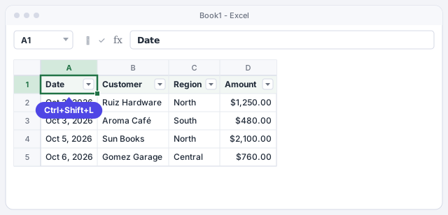
Filter by values: choose what to show
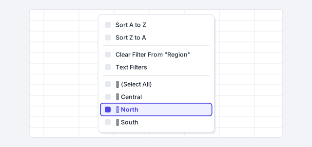
Click the arrow on Region. In the list at the bottom, clear (Select All) and check only North. Click OK. Three rows remain: Ruiz Hardware, Sun Books and Vida Pharmacy.
Notice two clues: the row numbers turn blue and skip (2, 4, 8…), and the arrow on Region changes to a funnel icon. That's how you know a filter is on. If the list is long, type in the menu's Search box instead of scrolling.
Filter by condition: amounts over $1,000
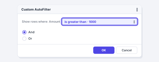
Now open the arrow on Amount and choose Number Filters › Greater Than…. In the Custom AutoFilter box, type 1000 and click OK.
Filters add up: you now see North sales over $1,000, that is, Ruiz Hardware ($1,250.00) and Sun Books ($2,100.00). Text columns offer Text Filters (Contains…, Begins With…) and date columns offer Date Filters (This Month, Last Month, Between…).
Total only what you see with SUBTOTAL
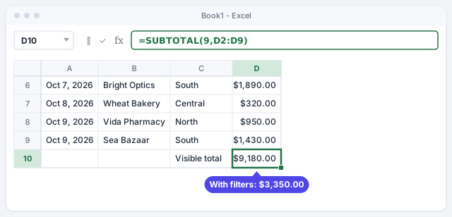
If you type =SUM(D2:D9), Excel also adds the rows hidden by the filter. To add only the visible ones, type in D10:
=SUBTOTAL(9,D2:D9)
The 9 tells SUBTOTAL to add. With no filters it returns $9,180.00; with the filters from the previous steps (North and over $1,000) it returns $3,350.00. Tip: if you click AutoSum under a filtered list, Excel writes SUBTOTAL for you.
Adds only visible rows: $9,180.00 with no filters and $3,350.00 with North and over $1,000.
Clear the filters when you're done
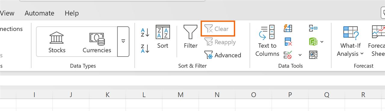
To clear the filter on a single column, open its arrow and choose Clear Filter From "Region". To clear every filter at once and keep the arrows, go to Data › Sort & Filter › Clear. To remove the arrows too, click Filter again or press Ctrl+Shift+L.
If you change data while a filter is on, click Reapply so the filter takes the new values into account.
Expert tips
- Keep the original order. Before sorting an important list, add a No. column with 1, 2, 3… When you want the starting order back, sort by that column smallest to largest.
- Sort by color. If you use conditional formatting to mark overdue invoices in red, in the Sort box change Cell Values to Cell Color and put red on top. The filter arrow also offers Filter by Color.
- A list that sorts itself. If you need a sorted or filtered copy that updates on its own, use formulas such as
SORTandFILTER(Microsoft 365 and Excel 2021): FILTER, SORT and UNIQUE. - Button filters for reports. If other people will filter the file, turn the list into a table and add slicers: big buttons that are easier to see and understand than arrows.
Common mistakes and how to fix them
After sorting, the amounts no longer match their customers.
Only one column was sorted with “Continue with the current selection”. Press Ctrl+Z right away and sort again by clicking a single cell, or choose “Expand the selection”.
When you sort, the header row gets mixed in with the data.
Open Data › Sort and check “My data has headers”. If the headers are formatted like the data, Excel sometimes doesn't recognize them: make them bold.
Only part of the list gets sorted or filtered.
An empty row or column is cutting the data region. Delete it, select the whole range before sorting, or turn the list into a table.
The total at the bottom doesn't change when you filter.
You're using =SUM(D2:D9), which also adds hidden rows. Replace it with =SUBTOTAL(9,D2:D9).
In Excel for Mac the buttons are on the same Data tab (Sort, Filter, Clear). The Sort box opens with ⌘+Shift+R, and filters turn on or off with ⌘+Shift+F or Ctrl+Shift+L.
Frequently asked questions
Does sorting or filtering delete data?
No. Sorting only changes the order of the rows and filtering only hides them. When you clear the filter, they all come back. The only irreversible thing is sorting wrongly and saving without undoing.
Why don't my dates sort correctly?
Because some are stored as text (they usually appear left-aligned). Excel sorts text character by character, not by date. Turn them into real dates; we explain how in number formats.
Can I sort in my own order, for example North, Central, South?
Yes. In Data › Sort, under Order, choose Custom List…, type North, Central, South, click Add and confirm.
Can I filter by two values in the same column, such as North or South?
Yes. In the filter list, check both North and South. For conditions on numbers or text, use Custom AutoFilter with Or between the two conditions.
Saved only in this browser.