Excel Tables: the format that makes filters, formulas and charts work on their own
Click any cell in your data and go to Insert › Tables › Table (or Home › Styles › Format as Table, or press Ctrl+T). Check the range, keep “My table has headers” selected and click OK. Then give it a name in Table Design › Table Name. From then on, filters, formatting, formulas and charts expand automatically every time you add a row.
It happens every month: you add ten new rows to your sales list and the total at the bottom doesn't include them, the chart stops short and the formula you copied down ends three rows early. You drag again, fix ranges and hope for the best.
An Excel table is a range of cells you've told Excel is “a list with headers”. It's like going from a pile of loose sheets to a labeled binder: Excel knows where it starts and ends, what each column is called, and that anything you add underneath belongs to it. It isn't just colored formatting: it's structure.
In this guide you'll turn a plain list into a table, name it, create a column that calculates itself, add a total row and use the table in formulas that never fall short.
What you'll learn
- How to turn a list into a table with Insert › Table or Ctrl+T
- Why you should give the table a name (and how)
- How to create calculated columns and an automatic total row
- How to write formulas with structured references such as
=SUM(Sales[Total])
Step by step
Get your data into a clean list
Before creating the table, check three things: a single header row at the top (a different name for each column), no completely empty rows or columns in the middle and no merged cells. In the example you have a product list in A1:C5 with the columns Product, Units and Price, plus a Total column that's still empty.
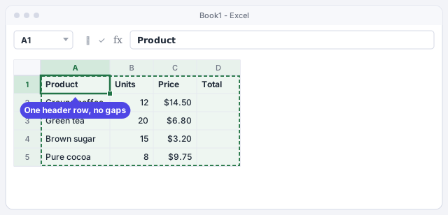
If the data came from an AI or another program, first delete any decorative title rows above the headers.
Create the table from Insert › Table
Click any cell in the list (you don't need to select all of it). Go to Insert › Tables › Table. You can also use Home › Styles › Format as Table, which lets you pick the colors as well, or the shortcut Ctrl+T.
Both routes create exactly the same thing: an Excel table. The only difference is the color style it starts with.
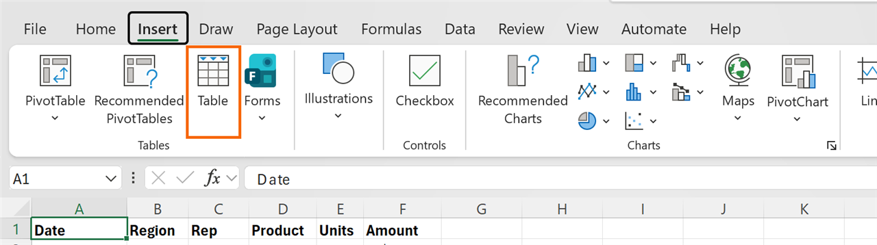
Confirm the range and check “My table has headers”
The Create Table box opens. Under Where is the data for your table? Excel already suggests the range ($A$1:$D$5). Make sure it covers every row and column, keep My table has headers selected and click OK.
Instantly you get banded rows, filter arrows on every header and a new tab on the ribbon: Table Design.

If you clear “My table has headers”, Excel adds a row of generic names (Column1, Column2…) and treats your real headers as data.
Give it a name that makes sense
Excel calls the table Table1. Change it: with a cell in the table selected, go to Table Design › Properties › Table Name, type Sales and press Enter.
The name can't contain spaces or start with a number. It's worth it: reading Sales[Total] in a formula is much clearer than Sheet1!D2:D5, for you, for your colleagues and for any AI you ask for help.

Write a formula once and let it fill the column
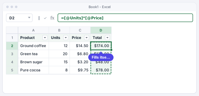
Click D2, type =, click B2, type * and click C2. Excel doesn't write B2*C2 but =[@Units]*[@Price]: the @ means “from this row”. Press Enter.
The formula copies itself down to the end of the table. This is called a calculated column: one formula for the whole column, no dragging.
Multiplies units by price on the same row and fills the whole column.
Add rows by typing right below
Type a new product in the first empty row under the table (in the example, A6: Cookies, 10 units, $4.60). When you press Enter or Tab, the table expands: the new row takes the formatting, the filter arrows include it and the Total column calculates $46.00 without you copying anything.
Another way: go to the last cell of the last row and press Tab; Excel creates a new row inside the table.
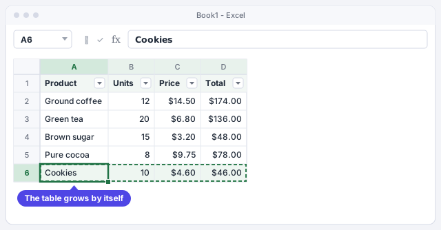
If the table doesn't expand, you probably left an empty row between the table and the new data. Always type in the row directly below.
Turn on the total row
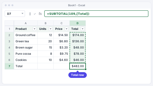
Go to Table Design › Table Style Options and check Total Row. A Total row appears at the bottom with the sum of the last column: $482.00. Excel writes =SUBTOTAL(109,[Total]) for you.
Click any cell in that row and you'll see an arrow: from there you pick Sum, Average, Max or a count for each column. Best of all, SUBTOTAL only counts visible rows, so the total changes when you filter.
Excel creates it for you: sums the Total column, ignoring hidden or filtered rows.
Use the table in formulas that never fall short
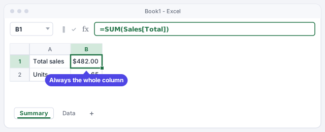
On another sheet (for example, Summary), type =SUM( and select the table's Total column. Excel writes =SUM(Sales[Total]). That reference means “the whole Total column of the Sales table”, however many rows it has: today it adds up to $482.00 and tomorrow it will include the new rows without touching the formula.
The same goes for charts and PivotTables built from the table: when you add rows, they update with it (PivotTables, when you click Refresh).
Adds the whole Total column of the Sales table, even as it grows.
Total units sold: 65 in the example.
Expert tips
- Headers always in view. If you scroll down a long table with a table cell selected, the column letters (A, B, C…) are replaced by your header names. For lists that aren't tables, use Freeze Panes.
- Ask the AI for readable formulas. Tell ChatGPT “my table is called Sales and has the columns Units, Price and Total” and ask for the formula with structured references. You'll get something like
=SUM(Sales[Total]), easy to check at a glance. - Remove duplicates without leaving the table. Under Table Design › Tools you'll find Remove Duplicates, Summarize with PivotTable and Insert Slicer (one-click filter buttons: slicers).
- A table is the best source for a PivotTable. If you build the PivotTable on the
Salestable, after adding rows you only need to click Refresh; no need to change the data source.
Common mistakes and how to fix them
The table stops halfway down the list or leaves columns out.
There was an empty row or column in the middle. Delete it or, if you already created the table, use Table Design › Properties › Resize Table to set the right range.
You type a different formula in one cell of the calculated column and a green triangle appears.
Excel is warning you that the cell doesn't match the column's formula. If it was a mistake, press Ctrl+Z. A calculated column should have the same formula on every row.
You want a normal list again, but after Convert to Range the colors stay.
Convert to Range removes the structure, not the style. Before converting, open the Table Design › Table Styles gallery and choose Clear, or apply a style with no colors.
In Excel for Mac the path is the same: Insert › Table or Home › Format as Table, and the shortcut is ⌘+T (Ctrl+T also works). The table name and total row are set on the table's contextual tab, which appears when you click inside it.
Frequently asked questions
What's the difference between an Excel table and a range with borders and colors?
A formatted range just looks nice. A table also knows where it starts and ends: it expands when you add rows, fills column formulas, comes with filters and lets you use names like Sales[Total] in formulas.
What does the @ in =[@Units]*[@Price] mean?
It means “the value on this same row”. [@Units] is the cell in the Units column on the row where the formula sits. Without the @, Sales[Units] refers to the whole column.
Does this work in older versions of Excel?
Yes. Tables have existed since Excel 2007 and the @ syntax since Excel 2010. Everything in this guide works in Excel 2016, 2019, 2021 and Microsoft 365.
Should I use Ctrl+T or Ctrl+L?
In English-language Excel for Windows both open the Create Table box. Ctrl+T is the easier one to remember, and it's also the one that works on Mac.
Saved only in this browser.