Pivot tables in 5 minutes: summarize thousands of rows without writing formulas
A pivot table summarizes a long list without formulas. Click inside your data, go to Insert › Tables › PivotTable, leave New Worksheet selected and click OK. In the PivotTable Fields pane, drag a text field (for example, Region) to the Rows area and a number field (Amount) to the Values area: Excel groups and totals each region instantly.
It happens every month: you have a sheet with hundreds of sales and someone asks “how much did we sell by region?”. You filter, add up, write it down, change the filter… and by the third region you no longer trust your numbers.
A pivot table is a summary Excel builds for you. You tell it what to show in the rows (regions), what in the columns (products) and which number to add up (the amount), and Excel groups and totals everything in a second. Think of it as sorting receipts into piles: one pile per region, with the total on top of each pile.
In this guide you build your first pivot table with a small example (eight sales, so you can check the math by hand). Eight rows or eighty thousand, it works exactly the same way.
What you'll learn
- How to prepare your data so the pivot table works the first time
- How to create it and place fields in Rows, Columns and Values
- How to switch from Sum to Count or Average and apply a currency format
- How to refresh it when the data changes or grows
Step by step
Set up your data as a clean list
A pivot table needs a list: one row per record (each sale) and one column per field (Date, Region, Salesperson, Product, Amount). Each column has a unique header in the first row, with no merged cells, no blank rows in the middle and no hand-typed subtotals.
Ideally, turn the list into an Excel table: click any cell in the data and go to Insert › Tables › Table. Then name it in Table Design › Table Name, for example Sales. That way, when you add rows, the pivot table picks them up on refresh. More in Excel Tables.
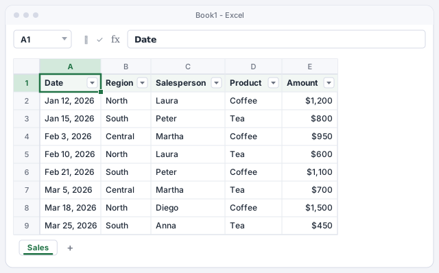
If the amount column mixes numbers with text (a “pending”, or figures pasted as text) or has blank cells, the pivot table will count it instead of summing it.
Insert the pivot table from the Insert tab
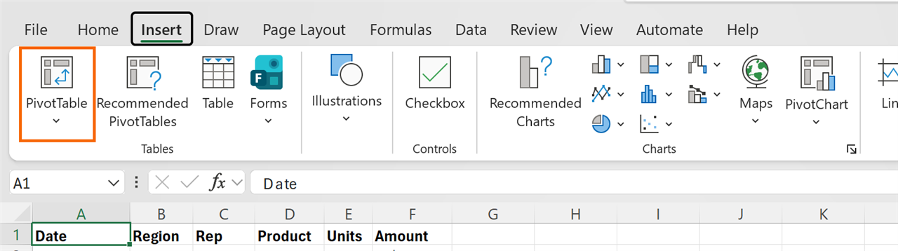
Click any cell in the Sales table (no need to select all of it). Go to Insert › Tables › PivotTable. In Microsoft 365 the button has an arrow: if you open the menu, choose the table or range option; the other sources (external data, Data Model, Power BI) are for advanced cases.
Next to it you'll see Recommended PivotTables, which suggests ready-made summaries. Today you'll build it by hand so you understand how it works.
Choose where the data comes from and where the summary goes
The PivotTable from table or range dialog opens (in some Microsoft 365 builds the title is slightly different, but the options are the same). Check that Table/Range shows Sales or a range such as Sales!$A$1:$E$9.
Leave New Worksheet selected: it's the tidiest option, because the summary doesn't mix with the data. Click OK. Excel creates a new sheet with an empty placeholder on the left and the PivotTable Fields pane on the right.
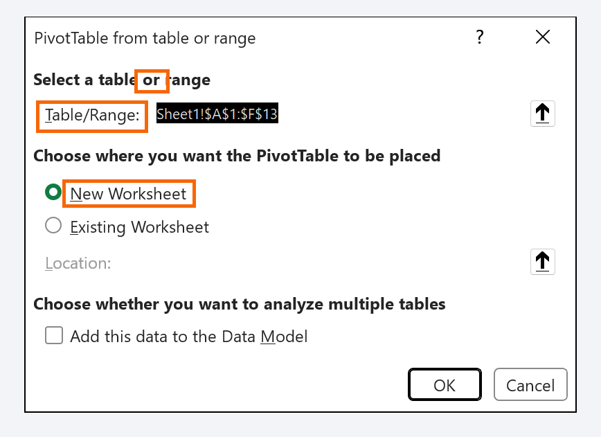
Leave “Add this data to the Data Model” unchecked: you only need it to relate several tables, and in that mode classic calculated fields aren't available.
Drag the fields to Rows and Values
At the top of the pane you see the field list: those are your column headers. Below are four areas: Filters, Columns, Rows and Values. Drag Region to the Rows area and Amount to the Values area.
The rule that keeps you on track: Rows and Columns hold the fields you want to group by (text or dates); Values holds what you want to calculate (usually numbers). If you tick a field's checkbox instead of dragging, Excel decides for you: text goes to Rows and numbers to Values.

Read the result and check one total by hand
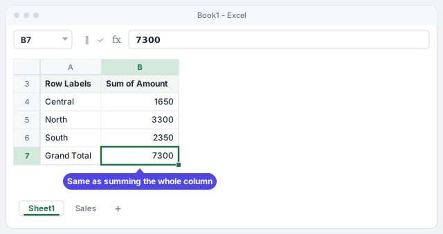
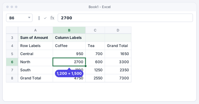
The summary appears on the left: one row per region and the sum of its sales. Central adds up to 1,650 (950 + 700), North to 3,300 and South to 2,350. The last row, Grand Total, shows 7,300: the same as =SUM(Sales[Amount]).
That's the expert habit: the first time, check one total by hand. If it matches, you can trust the rest.
Add a second dimension in Columns
Now drag Product to the Columns area. The table becomes a cross-tab: regions down the side, products across the top and, at each intersection, the total of those sales. For example, Coffee in the North adds up to 2,700 (1,200 + 1,500).
Try swapping them: Product to Rows and Region to Columns. That's why it's called a “pivot” table: you reshape the report in seconds without touching the data. To see a single salesperson, drag Salesperson to Filters and pick a name from the drop-down above the table.
Change the calculation and the number format
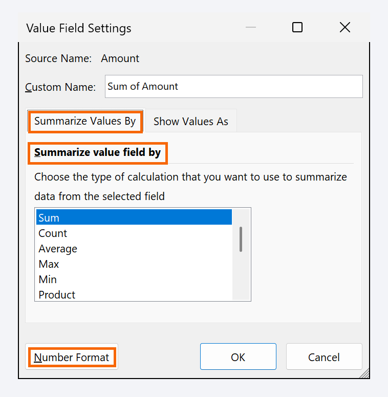
Click any number in the pivot table and go to PivotTable Analyze › Active Field › Field Settings (or right-click a number › Value Field Settings…). On the Summarize Values By tab, choose a different calculation: Count (how many sales) or Average (the average sale).
In the same dialog click Number Format and choose Currency with two decimals. The format applies to the whole field and sticks when you rearrange or refresh the table.
Refresh the pivot table when the data changes
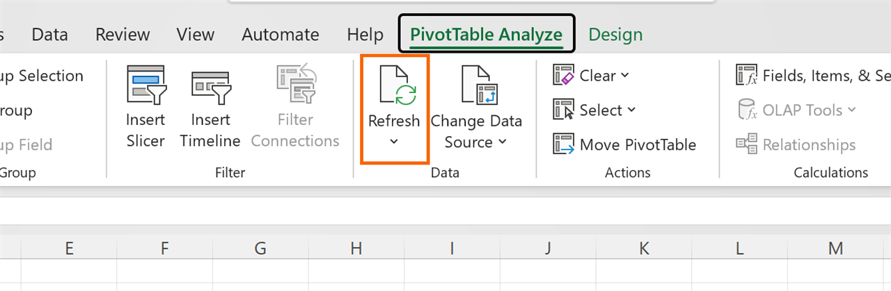
A pivot table doesn't recalculate on its own like a formula: it works from a copy of the data. If you change an amount or add sales to the Sales table, click inside the pivot table and go to PivotTable Analyze › Data › Refresh, or right-click it and choose Refresh. If you have several, open the Refresh arrow and choose Refresh All.
If your source was a plain range (not an Excel table) and you added rows below it, use Change Data Source to extend the range. With an Excel table you don't need to.
Expert tips
- Double-click a total. Excel creates a new sheet with the exact rows behind that number. Perfect for answering “where does this 3,300 come from?”.
- Drag the same field twice. Put Amount in Values as a sum and again as a count: you'll see the total and the number of sales side by side. For percentages and dates grouped by month, continue with pivot tables in depth.
- Sort by the number, not the name. Right-click an amount › Sort › Sort Largest to Smallest: your best-selling region moves to the top.
- Add filter buttons. With PivotTable Analyze › Filter › Insert Slicer you filter by region or salesperson in one click. We cover it in slicers and timelines.
- Use AI for the layout, not the math. Ask ChatGPT or Copilot “which fields should go in rows and values to see X”, then build it yourself: Excel does the calculating and doesn't make up numbers. You can also try Home › Analyze Data, which suggests summaries based on your data.
Common mistakes and how to fix them
The field shows up as “Count of Amount” instead of “Sum of Amount”.
The column has blank cells or text (for example, numbers pasted as text). Fix the source, refresh the pivot table and switch the calculation to Sum in Value Field Settings.
You added new sales and the total doesn't change.
Pivot tables don't refresh on their own: right-click › Refresh. If the source is a plain range, extend it with PivotTable Analyze › Change Data Source, or convert it to an Excel table.
The same region appears twice, as if they were different.
It's almost always a trailing space (“North ”). Clean it with =TRIM(B2) or Find and Replace, then refresh the pivot table.
In Excel for Mac the path is the same: Insert › PivotTable opens the PivotTable from table or range dialog (Create PivotTable in older versions), and the PivotTable Fields pane has the same four areas. The contextual tab is also called PivotTable Analyze; to switch Sum to Count, Control+click (or right-click) a number.
Frequently asked questions
How many rows can a pivot table summarize?
As many as fit on a worksheet (just over a million). If you have more, or the data lives in several files, import it with Power Query and build the pivot table from the Data Model: Power Query step by step.
Does changing the pivot table change my original data?
No. The pivot table works from an internal copy (the cache). You can rearrange it, filter it or delete it without touching the Sales table.
Pivot table or SUMIFS?
A pivot table is faster for exploring and reshaping. A formula like SUMIFS is better when you need the result in a fixed cell of a report with its own layout. See SUMIFS and COUNTIFS.
Official sources
Microsoft documentation consulted for this guide.
Saved only in this browser.