Pivot tables in depth: group dates, % of total and calculated fields
To group dates, right-click a date in the pivot table › Group and select Months and Years. For percentages, right-click a value › Show Values As › % of Grand Total. For a margin, go to PivotTable Analyze › Calculations › Fields, Items, & Sets › Calculated Field and type the formula =Amount-Cost.
You already know how to build a pivot table with totals by region. But the report people actually ask for is different: sales by month, each region's share of the total, growth versus last month and the margin each area brings in. That's where many people copy the pivot table to another sheet and add formulas by hand… which break as soon as the table changes size.
The pivot table can do all of that itself, with three tools almost nobody uses: grouping (turning individual dates into months, or bundling regions into zones), show values as (the same number seen as a percentage, a change or a running total) and calculated fields (new columns built from a formula over other fields). You'll learn all three with the data from the basic guide plus a cost column.
What you'll learn
- Group dates by month and year, and group items by hand
- Show % of grand total and the change from the previous month
- Create a margin calculated field and know when it misleads
- Switch the report to tabular form, ready to copy or print
Step by step
Start with real dates and a cost column
Use an Excel table (here, Sales) with a Date column that holds real dates, not text that looks like dates, and a Cost column next to Amount. Create the pivot table with Insert › Tables › PivotTable and place Region in Rows and Amount in Values.
A quick way to spot fake dates: unless you changed the alignment, real dates line up on the right of the cell and text dates on the left.
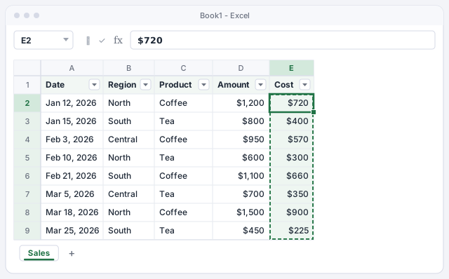
If the Date column has blank cells or dates stored as text, Excel won't let you group it by month.
Group dates by month and year
Put Date in the Rows area. In Microsoft 365, Excel often groups dates automatically; if you see individual dates, or want a different grouping, right-click any date in the pivot table and choose Group… (also under PivotTable Analyze › Group › Group Field).
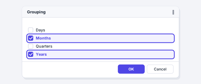
In the Grouping dialog, in the By list, click Months and Years so both are selected, then click OK. Always include Years if your data spans more than one year; otherwise January 2025 and January 2026 get added together into a single “Jan”. With the sample data you'll see Jan 2,000, Feb 2,650 and Mar 2,650: 7,300 in total.
With a number field in Rows, Group creates bands: for example, amounts from 0 to 499, 500 to 999, and so on.
Group items by hand: regions into zones
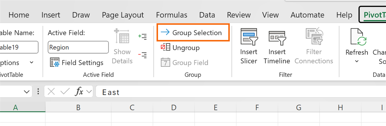
Grouping isn't only for dates. With Region in Rows, select the Central and North cells (Ctrl+click) and go to PivotTable Analyze › Group › Group Selection. Excel creates a group called Group1 and a new field, Region2, which appears in the field list.
Click the Group1 cell and type over it with any name, for example Inland Zone. The group totals 4,950 (1,650 + 3,300) and South stays at 2,350. To undo it, select the group and click Ungroup.
Show each region as a % of the total
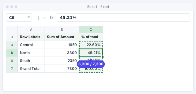
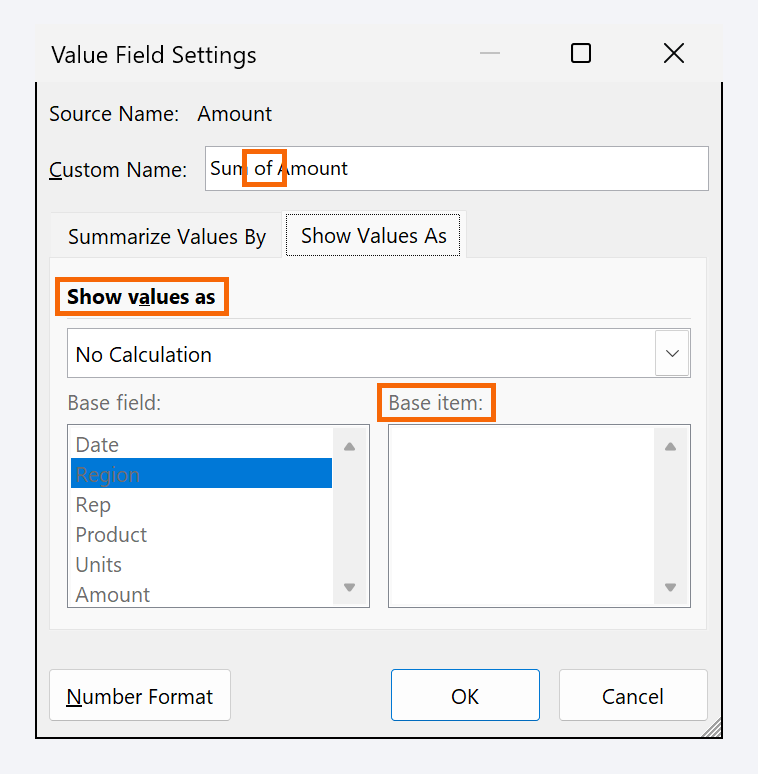
Drag Amount into the Values area a second time: you'll get two identical columns. Right-click a number in the second one and choose Show Values As › % of Grand Total (also available in Value Field Settings, on the Show Values As tab).
Rename the header by typing over it, for example % of total. Now you see the amount and its weight: North brings in 45.21% of sales. If you have products in Columns, try % of Row Total: you'll see how much of each region's sales is coffee and how much is tea.
Calculate the change from the previous month
With Date grouped by month in Rows, add Amount to Values once more and open Value Field Settings › Show Values As. Choose % Difference From; set Base field to Date and Base item to (previous). Click OK.
Each month is compared with the one before: February shows 32.50% (from 2,000 to 2,650) and March 0.00%. January is empty because it has no previous month to compare against. The same list also has Running Total In, for a year-to-date total.
Create a calculated field for the margin
A calculated field is a new pivot table column built from a formula over other fields. Click inside the pivot table and go to PivotTable Analyze › Calculations › Fields, Items, & Sets › Calculated Field….
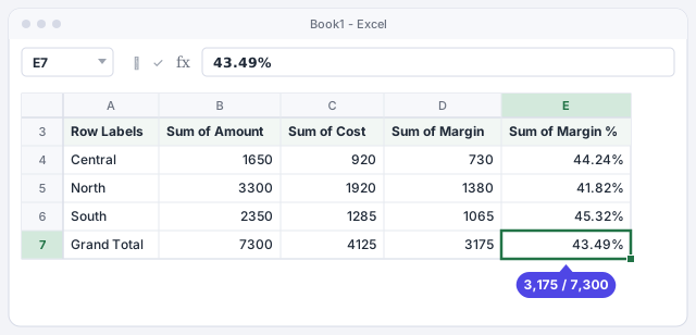
In Name type Margin. In Formula, clear the box and type =Amount-Cost (you can double-click fields in the list to insert them). Click OK: Sum of Margin appears in Values. Repeat with the name Margin % and the formula =(Amount-Cost)/Amount, and give it a percentage format.
Dollar margin for each group.
Margin on sales; apply a percentage format.

Check the result and understand how it calculates
With Region in Rows you'll see, for example, North: amount 3,300, cost 1,920, margin 1,380 and a 41.82% margin. The grand total shows a 3,175 margin on 7,300, which is 43.49%.
Watch out: a calculated field works on each group's sums, not row by row. For subtractions and percentages of sales that's exactly what you want (a region's margin % is its total margin divided by its total sales). But =Units*Price would give a wrong answer: it would multiply the sum of units by the sum of prices. Do that kind of calculation in a column of the source table.
Switch the report to tabular form
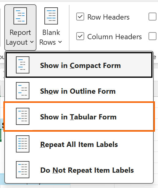
By default, a pivot table uses compact form: all row fields in a single indented column. For a report you'll copy, filter or print, go to the pivot table's Design tab › Report Layout › Show in Tabular Form. Each row field gets its own column, with its real name (Region, Date) instead of “Row Labels”.
In the same menu, Repeat All Item Labels fills the empty cells on the left, so every row makes sense on its own.
Expert tips
- Pull a number out with a formula. If you type
=in another cell and click a pivot table value, Excel builds something like=GETPIVOTDATA("Amount",$A$3,"Region","North"), which keeps returning 3,300 even when the table changes shape. If you'd rather get a normal cell reference, uncheck Generate GetPivotData under PivotTable Analyze › PivotTable › Options. - A header can't reuse a field name. If you want the column called Amount instead of Sum of Amount, type “Amount ” with a trailing space.
- Annoyed by automatic date grouping? In File › Options › Data there's a checkbox to turn it off for new pivot tables.
- Check what AI suggests. If Copilot or ChatGPT proposes a calculated field, verify one group with a calculator: the classic mistake is multiplying sums, as in step 7.
Common mistakes and how to fix them
When you try to group dates, Excel says it can't group the selection.
The source has blank cells or dates stored as text. Turn them into real dates (Data › Text to Columns, or =DATEVALUE(A2)), fill in the blanks and refresh the pivot table.
January from two different years is added together in one row.
You grouped by Months only. Open Group again and select Years as well.
The total margin % doesn't match the average of the regions' percentages.
That's correct: the calculated field divides total margin by total sales (3,175 / 7,300). A simple average of percentages ignores that each region sells different amounts.
In Excel for Mac, Group, Show Values As and calculated fields are on the PivotTable Analyze tab and in the shortcut menu (Control+click the pivot table). The dialog and option names are the same.
Frequently asked questions
Why does Excel group dates on its own without being asked?
Since Excel 2016, when you add a date field to a pivot table Excel can group it automatically by month (and year or quarter). Change the grouping with right-click › Group… or remove it with Ungroup.
Can I group by week?
Yes: in Grouping select only Days and type 7 as the number of days. Set the starting date to a Monday if you want Monday-to-Sunday weeks.
Calculated field or a column in the source data?
If the calculation is per row (amount = units × price), do it in the source. If it's a ratio between totals (margin, margin %, average price = amount ÷ units), a calculated field is perfect.
Can I show the percentage and the amount in the same pivot table?
Yes. Add the same field to Values twice and set Show Values As only on the second copy, as in step 4.
Official sources
Microsoft documentation consulted for this guide.
Saved only in this browser.