Charts people understand: pick the right type and remove the clutter
Select the data with its headers (leave out the total row) and go to Insert › Charts › Recommended Charts. Use columns to compare, lines for change over time and a pie only for a few parts of a whole. Then, on Chart Design, use Switch Row/Column if the series come out backwards and Add Chart Element to remove the legend and gridlines.
Someone asks for “a chart of sales” and Excel hands you six colors, a legend that adds nothing, gridlines everywhere and a title that says “Chart Title”. Nobody knows where to look. The problem isn't Excel: the chart was made before anyone decided what it had to say.
Think of a chart as a newspaper headline: it carries one idea and everything else is there to support it. In this guide you pick the chart type based on the question you want to answer, insert it in two clicks, fix the series when they come out backwards and remove everything that distracts. You'll end up with a chart your manager understands in five seconds and a title that updates itself.
What you'll learn
- Which chart type to use for what you want to show
- How to insert a chart with Recommended Charts and fix the series
- Which elements to remove so the chart reads on its own
- How to write a title that states the takeaway and updates with the data
Step by step
Prepare the data: headers, no blank rows, no total
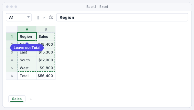
A chart is only as good as the range behind it. Keep one header row (Region, Sales), one row per item and no blank rows in the middle. A range is a block of cells, for example A1:B5.
Most important: don't select the total row. If you include it, you get a giant “Total” bar that flattens everything else. In the example, select only A1:B5. If you sort from largest to smallest before creating the chart, the bars come out already ranked and are much easier to read.
If you turn the data into an Excel table (Insert › Tables › Table), the chart grows automatically when you add new rows.
Choose the chart type based on the question
Before you click, answer this: what do I want the reader to see? This table covers 90% of cases:
| You want to show… | Use | Example |
|---|---|---|
| A comparison between categories | Columns (bars if the names are long) | Sales by region |
| Change over time | Lines | Monthly sales |
| Parts of a whole | Pie, with 4 or 5 slices at most | Budget breakdown |
| A relationship between two numbers | X Y (Scatter) | Price vs. units sold |
For our regions, the answer is Clustered Column: we're comparing four categories.
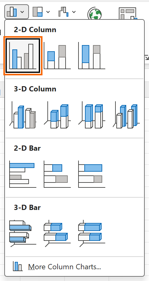
Avoid 3-D charts: they distort proportions and make one bar look bigger than it is.
Insert the chart with Insert › Recommended Charts
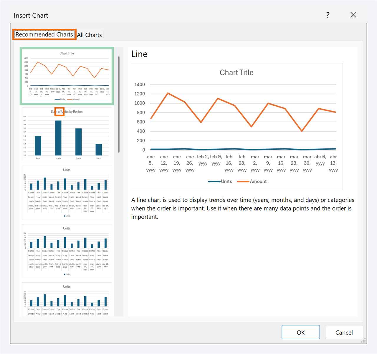
With A1:B5 selected, go to Insert › Charts › Recommended Charts. The Insert Chart window opens with several suggestions on the left and a preview using your real data. Choose Clustered Column and click OK.
If you already know what you want, you can go straight to the button for that type (column, line, pie) in the same Charts group. The All Charts tab shows the full catalog.
With the data selected, Alt+F1 instantly inserts a chart of the default type (columns) on the same sheet.
Fix the series with Switch Row/Column
When your data has several columns of numbers (for example, regions in rows and July, August and September in columns), Excel has to guess what goes on the horizontal axis and what goes in the legend. Sometimes it guesses wrong: you wanted to compare regions and it groups by month.
Click the chart and go to Chart Design › Data › Switch Row/Column. Rows become series and vice versa. If the range itself is wrong, use Select Data, in the same group, to add or remove series.
Remove the clutter with Add Chart Element
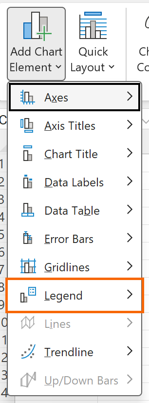
Now clean up. With the chart selected, go to Chart Design › Add Chart Element (or use the + button that appears next to the chart):
- Legend › None: with a single series, the legend says nothing the title doesn't.
- Gridlines: turn them off or make them very faint.
- Data Labels: put them above each column. Once you do, you can delete the vertical axis, because the number is already on the bar.
The expert rule: if an element doesn't help the main idea, it goes.
Write a title that states the takeaway (and updates itself)
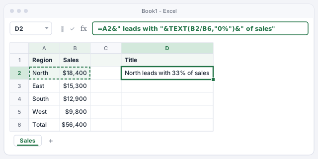
“Sales by region” describes; “North leads with 33% of sales” informs. To make the title change when the data changes, build it in a cell. In D2 enter the formula below: it joins the region name in A2 with its share of the total in B6 (18,400 / 56,400 = 33%).
Then click the chart title, click in the formula bar, type =, click cell D2 and press Enter. The title is now linked: if East takes the lead tomorrow, the chart says so on its own (as long as you keep the list sorted).
Joins the top region with its share of the total.
What the formula bar shows once the chart title is linked to D2.
Change the type without starting over
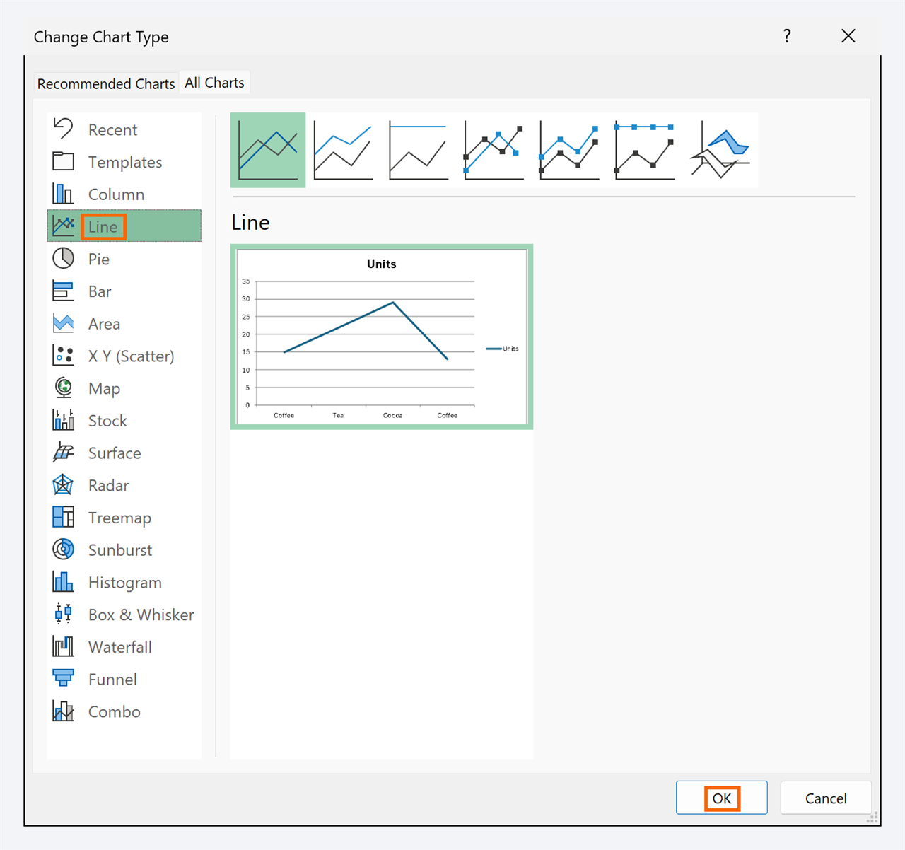
Realized the data is monthly and a line would work better? Don't delete anything. Select the chart and go to Chart Design › Type › Change Chart Type. Pick Line in the list on the left and click OK: the title, labels and colors that still make sense are kept.
This is also where you build a Combo chart: for example, sales as columns and margin as a line on a secondary axis, when the two series have very different scales.
Expert tips
- Highlight a single bar. Click the columns once (all get selected) and again on North (only that one). Go to Format › Shape Fill and give it a strong color; leave the rest gray. The eye goes straight to the takeaway.
- Rank horizontal bars. In a bar chart, Excel draws the first row at the bottom. Right-click the vertical axis › Format Axis and check Categories in reverse order so the largest sits on top.
- Save your design as a template. Once you have a clean chart, right-click › Save as Template…. You'll find it under Change Chart Type › Templates for every report.
- Let AI suggest, you decide. ChatGPT or Copilot can suggest a chart type, but check that it answers your question and doesn't include the total row.
- Several charts that filter together? That's the next level: a simple dashboard with a pivot table, a chart and a slicer.
Common mistakes and how to fix them
One huge column flattens all the others.
You included the total row in the range. In Chart Design › Select Data, fix the range so it ends on the last detail row (A1:B5 in the example).
A pie chart with twelve slices nobody can tell apart.
Use columns or bars sorted from largest to smallest. If you want to keep the pie, group the small slices into “Other” and keep 4 or 5 at most.
Dates or years show up as another series instead of on the axis.
Excel treated them as numbers. Leave the header cell of that column empty or turn them into text, or fix the series with Switch Row/Column and Select Data.
You add new rows and the chart doesn't show them.
The chart uses a fixed range. Turn the data into a table (Insert › Tables › Table) and create the chart again: from then on it grows by itself.
In Excel for Mac, Recommended Charts is on the Insert tab, and Switch Row/Column, Add Chart Element and Change Chart Type are on the Chart Design tab. To format an element, Control+click it and choose its format option. The Alt+F1 shortcut is Windows-only.
Frequently asked questions
Columns or bars?
It's the same chart turned on its side. Use columns by default and bars when category names are long (products, customers) or there are many of them: horizontally they read without tilting your head.
How do I make the chart update when I add data?
Build the chart from an Excel table. When you type a new row underneath, the table expands and the chart with it. We cover it in Excel tables: the format that makes filters, formulas and charts just work.
My title formula returns an error. Why?
Check the quotes: every piece of text must be inside straight double quotes, and each piece joined with &. If you copied it from a chat or a document, curly quotes are the usual culprit.
When should I use a combo chart?
When you want to compare two measures on very different scales, such as sales in dollars and margin as a percentage. Put one as columns and the other as a line on a Secondary Axis, from Change Chart Type › Combo.
Official sources
Microsoft documentation consulted for this guide.
Saved only in this browser.