Conditional formatting: let Excel highlight only what matters
Conditional formatting colors a cell only when it meets a condition, and the color updates by itself when the data changes. Select the range without headers and go to Home › Styles › Conditional Formatting › Highlight Cells Rules › Greater Than... Type the limit, pick a format and click OK. Edit rules later in Conditional Formatting › Manage Rules...
You have a list of sales, invoices or grades, and your manager only wants to know one thing: what's on track and what isn't? So you go row by row, coloring cells green or red by hand. The next day three numbers change… and the colors are no longer telling the truth.
Conditional formatting is like an automatic highlighter: you give it a rule ("color sales above $10,000 green") and Excel keeps watch for you. If the value changes, the color changes. You don't touch a thing.
In this guide you'll learn the quick rules that cover 90% of real cases: highlighting values, data bars, color scales, icons and duplicates. Plus how to manage and clear rules so your sheet doesn't turn into a rainbow.
What you'll learn
- Highlight cells above (or below) a limit in seconds
- When to use data bars, color scales or icon sets
- Find duplicate values without any formulas
- Edit, reorder and clear rules in the Rules Manager
Step by step
Select only the cells you want to evaluate
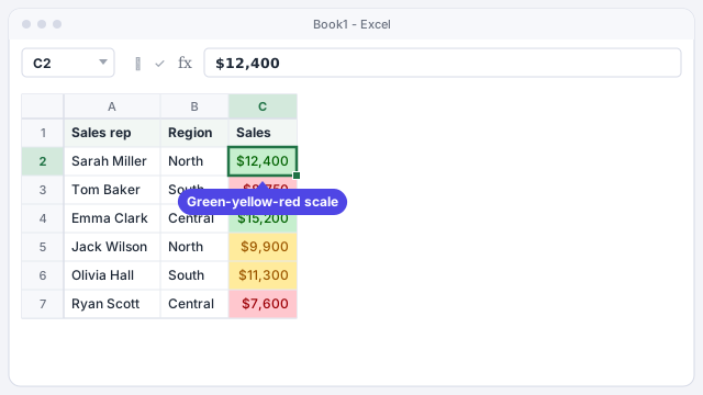
In the example you have quarterly sales for six sales reps. Select the numbers, C2:C7. A range is simply a block of adjacent cells.
Leave out the header (Sales) and any total row: the total would always exceed the limit and, in a color scale, it would distort every shade.
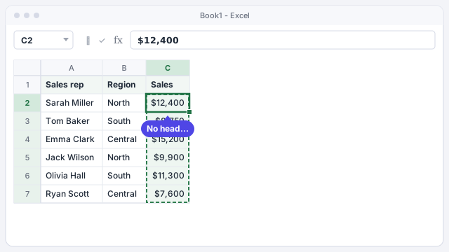
Open Home › Styles › Conditional Formatting
On the Home tab, in the Styles group, click Conditional Formatting. A menu opens with every family of rules: Highlight Cells Rules, Top/Bottom Rules, Data Bars, Color Scales and Icon Sets.

If your Excel window is narrow, the Styles group collapses into a single button: click it and you'll find Conditional Formatting inside.
Choose Highlight Cells Rules › Greater Than...
Point to Highlight Cells Rules and, in the submenu, choose Greater Than.... The same submenu has Less Than..., Between..., Equal To..., Text that Contains... and A Date Occurring... (for example, "last week").
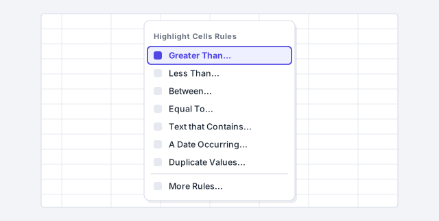
Type the limit and pick a format
In the Greater Than box type 10000 (no commas or dollar sign). In the with list, change the default (Light Red Fill with Dark Red Text) to Green Fill with Dark Green Text. Excel previews the result on the sheet as you choose. Click OK.
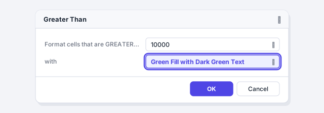
If you type a reference such as =$F$1 instead of a number, the limit lives in cell F1: change it and every color recalculates.
Check the result by changing a value
Sarah, Emma and Olivia turn green: they're the only ones above $10,000. Now the real test: change Tom's sales to 10500. His cell turns green instantly. That's the difference from coloring by hand: the rule does the work for you.
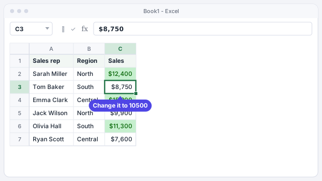
If a number above the limit doesn't change color, it's probably a number stored as text (it usually sits left-aligned). Convert it to a number and the rule will work.
Try data bars, color scales and icons
With the same range selected, open Conditional Formatting and try the other three families. Hover over each option to preview it:
- Data Bars: a bar inside each cell, proportional to its value. Great for comparing at a glance.
- Color Scales: a gradient (for example, green for high values, yellow for the middle and red for low). Perfect for heat maps.
- Icon Sets: arrows, traffic lights or flags depending on which third each value falls into.
Pick one per range. Bars, colors and icons all at once are harder to read than nothing.
Flag duplicates in one click
Select the invoice number column (A2:A6) and go to Home › Conditional Formatting › Highlight Cells Rules › Duplicate Values.... Accept the suggested format and invoice INV-1022, entered twice, turns red.
It's the fastest way to check a list before you send it or match it against another one.
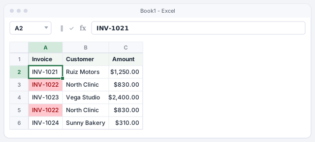
This rule only flags. To delete the repeated rows, use Data › Remove Duplicates after you've reviewed them.
Review, edit or clear rules
Go to Home › Conditional Formatting › Manage Rules.... In Show formatting rules for, choose This Worksheet to see them all. From here you can change a rule (Edit Rule...), the range it covers (the Applies to column) or the order: the rule on top wins when two clash.
To wipe everything: Conditional Formatting › Clear Rules › Clear Rules from Selected Cells or Clear Rules from Entire Sheet.

Expert tips
- Use the Quick Analysis button. When you select a range of numbers, a small icon appears at its bottom-right corner. Its Formatting tab offers bars, colors and icons with an instant preview.
- Apply the rule to a table. If your data is in an Excel Table, new rows pick up the conditional formatting without you extending the range.
- Filter by color. In a column with conditional formatting, the filter button offers Filter by Color: show only the green or red rows in one click.
- Copy rules with the brush. Home › Format Painter also copies conditional formatting to another range, so you reuse a rule without rebuilding it.
- Need to color whole rows or overdue dates? That takes a formula-based rule: see conditional formatting with formulas.
Common mistakes and how to fix them
You include the header or the total row in the range.
The total always stands out and squashes the color scale. Select only the data (C2:C7 in the example) or fix the range in Manage Rules › Applies to.
You copy and paste rows and end up with dozens of repeated rules.
Pasting formatted rows splits rules into fragments. Open Manage Rules with This Worksheet, delete the extras and keep one rule covering the full range.
A number above the limit doesn't change color.
It's stored as text. Convert it to a number (for example, with the green warning in the cell's corner › Convert to Number) and the rule will apply.
The sheet has so many colors nobody can read it.
One rule, one message. Remove anything that doesn't help a decision and use one type of formatting per column.
In Excel for Mac the Conditional Formatting button is also on the Home tab, with the same families of rules (highlight cells, top/bottom, data bars, color scales and icon sets). You review rules from Conditional Formatting › Manage Rules.
Frequently asked questions
Does conditional formatting change cell values?
No. It only changes how cells look. The numbers stay the same and any formulas that depend on them aren't affected.
Can I put several rules on the same range?
Yes. For example, green above $10,000 and red below $8,000. If two rules hit the same cell with clashing formats, the one higher up in Manage Rules wins.
How do I highlight the top 3 sales or those above average?
Use Conditional Formatting › Top/Bottom Rules. It has options for the highest or lowest values (you can change 10 to 3) and Above Average.... In the example the average is $10,858, so Sarah, Emma and Olivia would stand out.
Does the formatting survive if I send the file?
Yes. Rules are saved in the workbook and work in whatever Excel opens it, including Excel for the web.
Official sources
Microsoft documentation consulted for this guide.
Saved only in this browser.