Conditional formatting with formulas: highlight whole rows, overdue dates and duplicates
Select the full range starting on row 2 (for example A2:E8) and go to Home › Conditional Formatting › New Rule... › Use a formula to determine which cells to format. Write the formula for row 2 only, with $ before the column. For pending invoices past due: =AND($D2="Pending",TODAY()>$E2). Click Format..., pick a fill and click OK.
Quick conditional formatting rules color a cell based on its own value. But in real life you want something else: the whole row of an invoice turning red when it's unpaid and past due. That depends on two columns at once, and no menu rule does it.
The answer is a formula rule. Think of it as a yes-or-no question Excel asks on every row: "is this invoice pending and overdue?" If the answer is TRUE, it applies the format; if it's FALSE, it does nothing.
The only tricky part is the $ signs. In this guide you'll see why $E2 works and $E$2 doesn't, and you'll build three rules you'll use every week: overdue, due soon and duplicates.
What you'll learn
- The golden rule: write the formula for the first row of the range
- Why $E2 (locked column, free row) colors whole rows
- Highlight invoices that are overdue or due in the next 7 days with TODAY
- Flag duplicates with
=COUNTIF($A$2:$A$8,$A2)>1 and order your rules
Step by step
Get the idea: a question Excel repeats on every row
You select a range, write a formula that is true or false for the first row, and Excel mentally copies it to the rest, just like dragging a formula down. Wherever it returns TRUE, it applies the format.
The example is an invoice log: column D holds the status and column E the due date. Assume today is Oct 10, 2026.

Select the whole range, starting at A2
Click A2 and drag to E8. Leave the headers out. Notice the active cell (the white one inside the selection, shown in the Name Box) is A2: the formula you write is read from that cell's point of view.
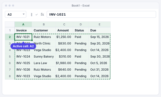
If you select from the bottom up, the active cell will be A8 and you'd have to write the formula for row 8. The safe habit is to always select from the top-left corner.
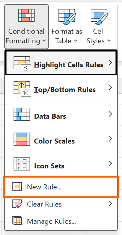
Open Home › Conditional Formatting › New Rule...
On the Home tab, in the Styles group, open Conditional Formatting and choose New Rule.... The New Formatting Rule dialog opens.
Choose the formula rule type and write the overdue rule
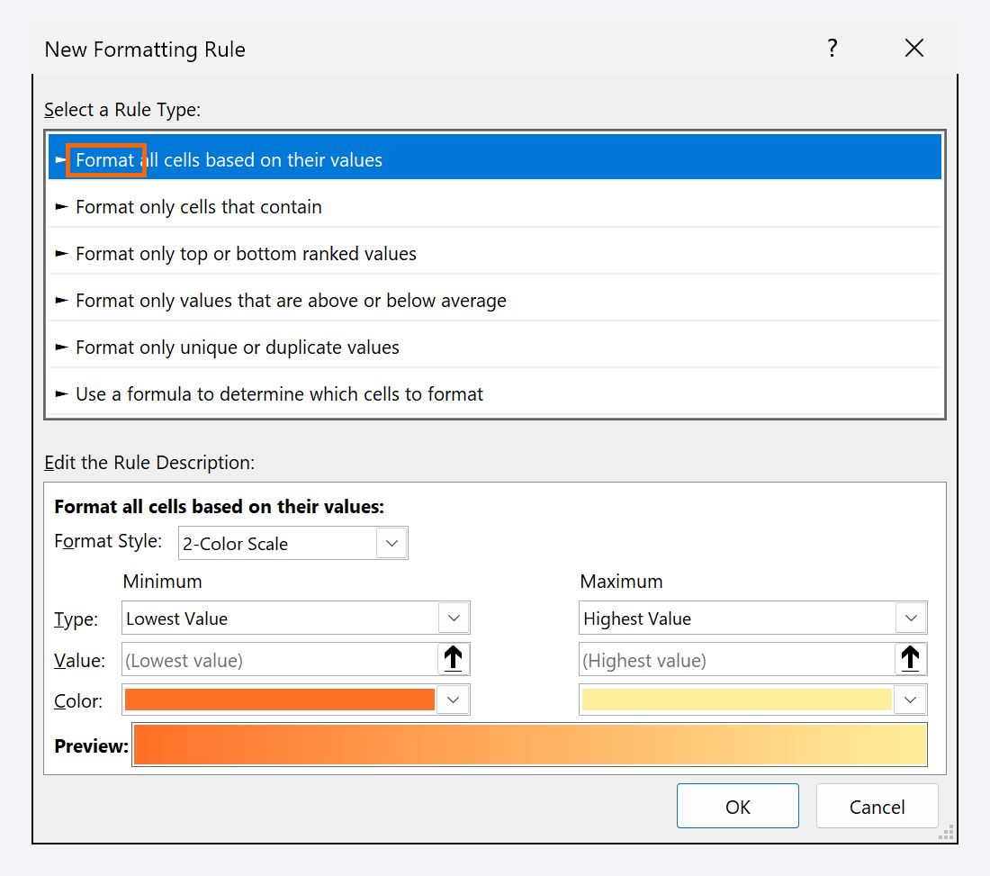
Under Select a Rule Type, choose the last option: Use a formula to determine which cells to format. In the Format values where this formula is true box, type:
=AND($D2="Pending",$E2<TODAY())
It reads: "this row's status is Pending and its due date is before today". AND only returns TRUE when both conditions are met, and TODAY returns the current date.
TRUE if the invoice on that row is pending and its due date has passed.
Click Format... and pick a fill
Click Format.... A slimmed-down Format Cells dialog opens with only four tabs: Number, Font, Border and Fill. On Fill, choose a soft red under Background Color. Click OK twice.
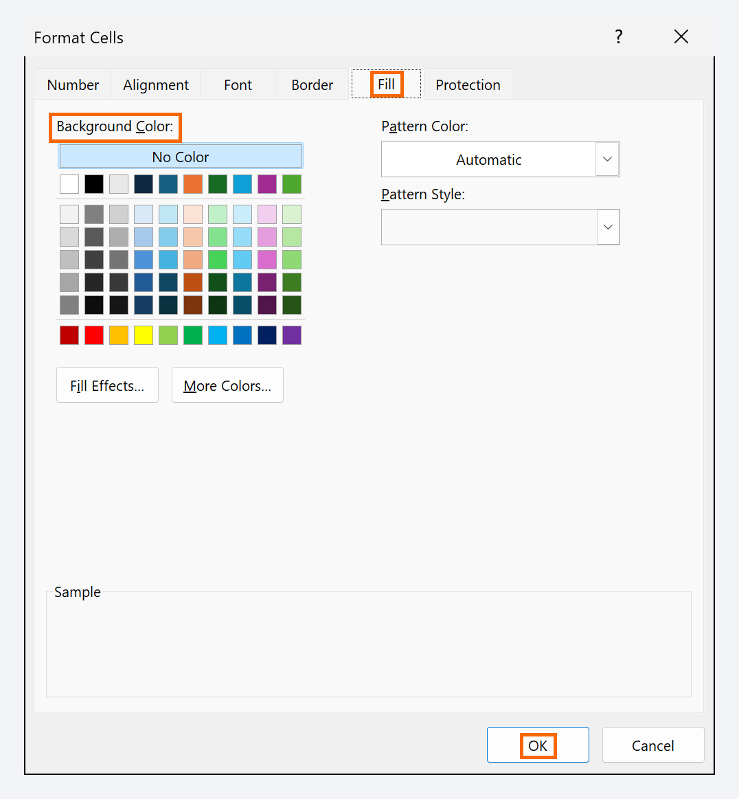
Pick light colors: the text must stay readable, including when printed in black and white.
Check the result and understand the $
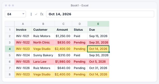
The rows for INV-1022 and INV-1025 turn red end to end: they're pending and overdue. INV-1024 is also past its date, but it's paid, so it stays white.
Why the whole row? Because the $ locks the column. Excel evaluates the formula in every cell, and every one of them looks at column E on its own row:
| You type | What happens |
|---|---|
$E2 | Locked column, free row: colors whole rows. Correct. |
E2 | Column B would look at F, column C at G… Only odd cells get colored. |
$E$2 | Every row looks at the same cell: everything gets colored, or nothing. |

Add a second rule: due in the next 7 days
With the same range A2:E8 selected, repeat New Rule... with this formula and a yellow fill:
=AND($D2="Pending",$E2>=TODAY(),$E2-TODAY()<=7)
Subtracting two dates gives the number of days between them. Both INV-1023 rows get flagged: they're due in 4 days. INV-1026 stays white: it has 21 days to go.
TRUE if it's pending and due today or within the next 7 days.
If you put the number of days in a cell (say H1) and use $E2-TODAY()<=$H$1, you can change the window without touching the rule.
Flag duplicate invoice numbers with COUNTIF
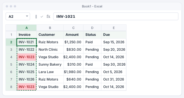
Select only A2:A8 and create another formula rule:
=COUNTIF($A$2:$A$8,$A2)>1
Here the range being counted is fully locked ($A$2:$A$8), because it's always the whole list; what changes on each row is the value being looked for ($A2). If it appears more than once, it's colored. INV-1023 was entered twice.
Counts how many times this row's number appears in the list; more than once means it's flagged.
Order and review your rules in Manage Rules
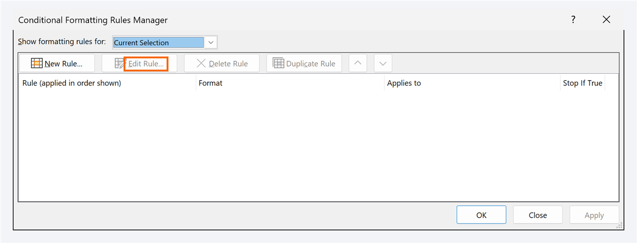
Go to Home › Conditional Formatting › Manage Rules... and, in Show formatting rules for, choose This Worksheet. You'll see your three rules with their formulas and ranges under Applies to. Use the arrows to change the order: if two rules give clashing formats to the same cell, the top one wins. The Stop If True box prevents the rules below from applying once a rule is met.
Expert tips
- Test the formula in a cell first. Type
=AND($D2="Pending",$E2<TODAY())inF2and drag it down. Wherever you seeTRUE, the row will be colored. Once it works, copy it into the rule and delete the helper column. - Banded rows without a table. The rule
=MOD(ROW(),2)=0colors even rows: the classic "zebra stripes" that make long lists easier to read. - Weekends on a calendar. If the date is in column
A,=WEEKDAY($A2,2)>5flags Saturdays and Sundays. - Ask AI for the rule, with context. Tell ChatGPT: "conditional formatting formula for range A2:E8, English Excel, color the row if D is Pending and E is before today". Then check it with the helper column. More in asking AI for formulas.
- Unsure about $? Review relative and absolute references: it's exactly the same logic.
Common mistakes and how to fix them
You click a cell while typing the formula and Excel inserts $E$2.
Clicking inserts an absolute reference. Remove the $ before the row so it reads $E2; otherwise the whole range gets colored, or nothing does.
The colors show up shifted by one row.
The formula doesn't match the active cell. If the range starts at A2, the formula must refer to row 2 ($E2), not row 1.
Pressing the arrow keys inside the formula box inserts strange references.
The box is in Enter mode and the arrows select cells. Press F2 to switch to Edit mode and move through the text.
The date rule flags nothing even though some invoices are overdue.
The dates are stored as text. Check that they're right-aligned and convert them into real dates.
In Excel for Mac the path is the same: Home › Conditional Formatting › New Rule. Choose the Classic style and the option to use a formula to determine which cells to format; the formula itself, $ signs and functions included, is identical.
Frequently asked questions
Can I use table references like Invoices[Due] in the rule?
Not directly: conditional formatting formulas don't accept structured references. Use regular references such as $E2; if the range is a table, new rows pick up the rule.
I copied a formula from a Spanish site and it fails. Why?
Spanish-language Excel uses semicolons and translated function names (Y, HOY). In English Excel use commas and AND, TODAY: =AND($D2="Pending",$E2<TODAY()).
Do the colors update by themselves every day?
Yes. TODAY recalculates when you open the workbook and whenever Excel recalculates, so an invoice moves from yellow to red without you doing anything.
Does this work in older versions of Excel?
Yes. Formula rules, AND, TODAY and COUNTIF work in Excel 2007 and later, and in Excel for the web.
Official sources
Microsoft documentation consulted for this guide.
Saved only in this browser.