Ask ChatGPT (or any AI) for formulas and check that they're right
To get a formula from an AI, describe your columns, the row range and the result cell, and say which Excel language and separator you use. Paste the formula in the first row, check three rows by hand (including an edge case) and, if something looks off, use Formulas › Formula Auditing › Evaluate Formula or select part of the formula and press F9.
You ask ChatGPT for a formula, paste it into Excel and get #NAME?. Or worse: no error, just a number… that nobody checks until someone spots the mistake in the report. AI helps a lot, but it can't see your sheet, doesn't know your Excel setup and sometimes invents functions with total confidence.
Think of the AI as an expert colleague helping you over the phone: if you don't describe the sheet well, it guesses. In this guide you'll learn what to tell it, how to get a formula that's ready to paste, and how to verify it in two minutes.
What you'll learn
- What information to give the AI so it gets the formula right the first time
- How to ask for the right function names and separator for your Excel
- How to check a formula with three rows by hand, Evaluate Formula and F9
- Typical AI mistakes: invented functions, wrong ranges and missing $ signs
Step by step
Describe your sheet before you ask
The AI can't see your file. Tell it what's in each column, which rows the data starts and ends on, and which cell you want the result in. A range is a group of cells, such as D2:D200: give exact ranges, not “the amounts column”.
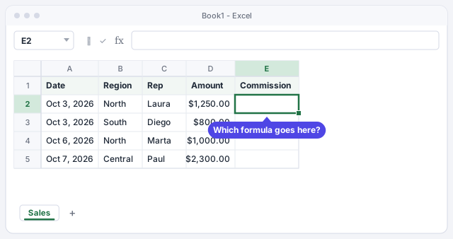
In the example you have a Sales sheet with the date in A, the region in B, the sales rep in C and the amount in D, from row 2 to row 200. In column E you want the commission: 5% if the amount is over $1,000, and 2% otherwise.
If the data is confidential, don't paste the sheet into the chat: describe the columns and add two or three made-up rows as an example.
Tell the AI your Excel language and separator
Most AIs answer with English function names and commas between arguments. That works in English Excel with US regional settings. But if your Excel is in another language, or your regional settings use a comma for decimals (common in Europe and Latin America), Excel expects translated names and semicolons. Say so in the prompt: “I use Excel in English with commas as the argument separator”.
Excel translates formulas already in a cell when a file opens in another language, but a formula pasted as text from a chat is never translated. Decimals matter too: with US settings, write 0.05, with a point.

If Excel rejects a formula that looks fine, look at a formula that already works in your sheet and ask the AI for that same separator.
Write the complete prompt
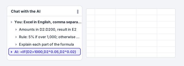
Put everything into one prompt: the data, the exact rule, the result cell, your Excel setup and an instruction to explain the formula piece by piece. That explanation will help you check it.
| Weak prompt | Prompt that works |
|---|---|
| Give me a formula for the commission | I use Excel in English. Amounts are in D2:D200. In E2 I want the commission: 5% if the amount is greater than 1,000, otherwise 2%. Use commas as separators. Explain each part. |
| Add up the North sales | Regions are in B2:B200 and amounts in D2:D200. In H2 I want the total for the region typed in G2, and I'll copy the formula down to H4. Lock the ranges with $. |
Paste the formula in the first row and copy it down
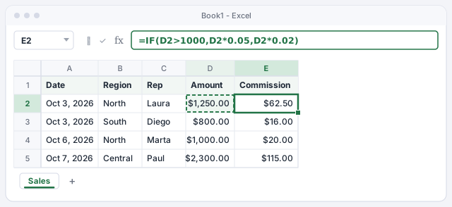
Click E2, paste the formula and press Enter. Then copy it to the other rows: double-click the small square at the bottom-right corner of the cell (the fill handle) or drag it down.
The formula =IF(D2>1000,D2*0.05,D2*0.02) says: “if the amount in D2 is greater than 1,000, multiply it by 0.05; otherwise by 0.02”. When you copy it, Excel changes D2 to D3, D4… on each row, which is exactly what you want here.
5% commission if the amount is over 1,000; otherwise 2%.
If your data is in an Excel table, the formula fills the whole column automatically.
Check three rows by hand
Getting numbers doesn't mean they're right. Pick three rows and work out the result with a calculator: one that meets the condition, one that doesn't, and an edge case, right on the boundary.
- Row 2: $1,250 is over 1,000, so 1,250 × 0.05 = $62.50. Correct.
- Row 3: $800 isn't over 1,000, so 800 × 0.02 = $16.00. Correct.
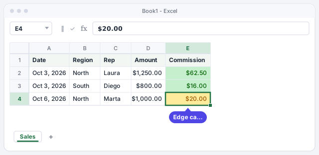
- Row 4: exactly $1,000. The formula returns $20.00 (2%), because 1,000 is not greater than 1,000.
The edge case is where people and AIs get it wrong most often. If your rule was “$1,000 or more”, change > to >=: =IF(D2>=1000,D2*0.05,D2*0.02).
Step through the formula with Evaluate Formula
For long formulas, let Excel show you the calculation. Select the cell and go to Formulas › Formula Auditing › Evaluate Formula. Click Evaluate several times: Excel replaces each part with its value (first D4 with 1000, then the comparison with FALSE…) until it reaches the result. You'll see the exact point where the formula departs from what you expected.

Trace Precedents, in the same group, draws arrows to the cells the formula uses: you'll see at a glance whether it points to the right column.
Calculate just one part of the formula with F9
An expert trick: click the cell and, in the formula bar, select just a piece, for example D4*0.02. Press F9: Excel shows the result of that part (20). Press Esc to leave without changing anything. It works with any complete part: a condition, a range or a function with its parentheses.

If you press Enter instead of Esc, the selected piece is replaced by its value and the formula stops updating. If that happens, press Ctrl+Z.
Fix the typical AI mistakes
When something goes wrong, it's almost always one of these:
- Names Excel doesn't recognize.
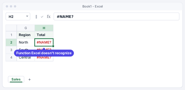
#NAME?means an unknown function: one from Google Sheets (such asQUERY), a name in another language, or an invented one likeSUMIFDATE. Look it up in Formulas › Function Library › Insert Function. - Wrong ranges. If the AI uses
D2:D100and your data runs to row 200, the missing rows aren't counted, with no warning. - References without
$. If the ranges shift when you copy down, it's missing absolute references. Click the reference and press F4 to add the$signs. - New functions.
XLOOKUP,FILTERandLETonly exist in Microsoft 365 and Excel 2021 or later. On an older Excel, ask for an alternative such asINDEXandMATCH.
Total for the region typed in G2; the $ signs lock the ranges when you copy it down.
Expert tips
- Ask for the explanation, not just the formula. Add “explain each part in one sentence”. If the explanation doesn't match your rule, neither does the formula.
- Give examples with the expected result. “1,250 should give 62.50; 800 should give 16”. The AI can check itself against them, and you already have your control rows.
- Tell it which error you see. If you get
#VALUE!or#N/A, say which error appears and on which row: it usually fixes it. We explain each error in formula errors. - Work with Excel tables. With a table named Sales, the AI can write
=SUM(Sales[Amount]), which is easier to read and never falls short when you add rows. See how in Excel tables.
Common mistakes and how to fix them
You paste the formula and Excel shows #NAME?.
There's a function from Google Sheets, from another language version or simply invented. Ask the AI for a version for your Excel, or find the correct name in Formulas › Insert Function.
The formula returns a result, but the total doesn't add up.
Check the ranges: the AI may have used a range shorter than your data or the wrong column. Use Trace Precedents to see which cells it points to.
When you copy the formula down, the results go wrong.
It's missing absolute references. Lock the ranges that mustn't move with $ (the F4 key), such as $D$2:$D$200.
In Excel for Mac, Evaluate Formula and Trace Precedents are on the same Formulas tab. To add $ signs to a reference you can use ⌘+T. Function names and the separator depend on the language and regional settings, just as on Windows.
Frequently asked questions
Why does my colleague's Excel show different function names?
Excel displays function names in its own language and uses the separator from the regional settings. A formula typed in a cell is translated automatically when the file opens in another language, but text pasted from a chat is not.
Can I paste my real data into ChatGPT?
Avoid it with personal, customer or confidential data, and follow your company's policy. To get a formula, describing the columns and giving two or three made-up rows is enough.
How do I know whether a function exists in my Excel?
Type = and the first few letters in a cell: Excel suggests only the functions available in your version. If it isn't in the list, your Excel doesn't have it.
Saved only in this browser.