Formula errors (#N/A, #VALUE!, #REF!, #DIV/0!): what they mean and how to fix them
Each Excel error points to a cause: #DIV/0! is a division by zero or by an empty cell; #N/A, a lookup that can't find the value; #VALUE!, text where a number was expected; #REF!, a deleted cell or column; #NAME?, a misspelled function or text without quotes. Track the cause with Formulas › Formula Auditing › Evaluate Formula and use IFERROR only for errors you expect.
It happens right before you send the report: you open the sheet and, instead of numbers, you see #N/A, #VALUE! or #REF!. Even worse if ChatGPT gave you the formula and you have no idea where to start. The temptation is to delete it and type the number by hand. Don't.
An Excel error isn't a random glitch: it's a message with a clue. It works like the warning lights on a car dashboard: each symbol means a different problem, and if you can read it, you know where to look. #DIV/0! isn't fixed the same way as #N/A.
In this guide you learn what each error means, the most common cause of each one, how to find it with the auditing tools and when it makes sense to hide it with IFERROR.
What you'll learn
- What #DIV/0!, #N/A, #VALUE!, #REF! and #NAME? mean
- The most common cause of each error and how to fix it
- How to use Evaluate Formula to see which part of a formula fails
- When to use IFERROR or IFNA and when not to
Step by step
Identify the error and read Excel's clue
Click the cell with the error. A warning icon appears next to it: hover over it and Excel tells you what kind of problem it sees. This table is your cheat sheet:
| Error | What it means | Most common cause |
|---|---|---|
#DIV/0! | Division by zero | Dividing by an empty cell or a 0 |
#N/A | Value not available | A lookup can't find what it's looking for |
#VALUE! | Wrong type of data | Text where there should be a number |
#REF! | Invalid reference | A row, column or sheet the formula used was deleted |
#NAME? | Unknown name | Misspelled function or text without quotes |
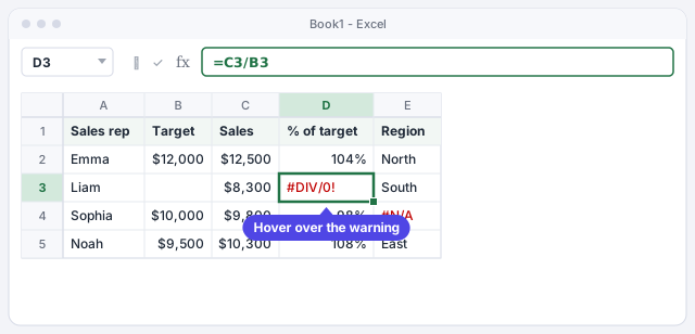
Fix #DIV/0!: avoid dividing by an empty cell
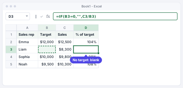
Liam doesn't have a target yet, and to Excel an empty cell is worth 0. Dividing 8,300 by 0 is impossible, hence the error. You have two options: fill in the missing figure or make the formula wait until it's there. Type =IF(B2=0,"",C2/B2) in D2 and copy it down: if there's no target, the cell stays empty; if there is one, it calculates the percentage.
Leaves the cell empty while there's no target; otherwise, divides.
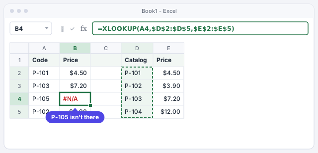
Fix #N/A: check that the lookup value exists
#N/A almost always comes from a lookup (XLOOKUP, VLOOKUP, MATCH) that can't find the value. Here the code P-105 isn't in the catalog. Before covering it up, check three things: that the code really exists, that it has no extra spaces ("P-105 " isn't the same as "P-105") and that you're not mixing numbers with numbers stored as text.
If it's normal for some codes to be missing, use the fourth argument of XLOOKUP to show a clear message.
If the code isn't in the catalog, shows Not found instead of #N/A.
To strip invisible spaces from a column of codes, use =TRIM(A2) in a helper column and paste the result as values.
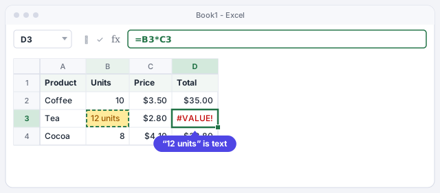
Fix #VALUE!: find the text hiding among the numbers
On the tea row someone typed 12 units instead of 12. To Excel that's text, and you can't multiply text by a price. Leave just the number in the cell (if you want to see “units”, add it with a custom number format). Other typical causes: odd spaces that come from copying from a website or a PDF, or dates typed as text.
To check whether a cell holds a real number, type =ISNUMBER(B3): if it returns FALSE, it's text.
TRUE if B3 is a number; FALSE if it's text.
SUM ignores text cells without warning: =SUM(B2:B4) won't show an error, but the total will be wrong. Check your data even if you don't see #VALUE!.
Fix #REF!: undo the deletion or use ranges
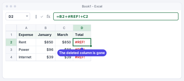
Each expense total was =B2+C2+D2 (January, February and March). When you deleted the February column, the formula lost one of its cells and now reads =B2+#REF!+C2. The fastest fix is to undo right away with Ctrl+Z. If it's too late, rewrite the formula: =SUM(B2:C2).
To stop it happening again, use ranges instead of adding cell by cell: if the total had been =SUM(B2:D2), Excel would have adjusted the range by itself when you deleted the column.
A range adapts when you delete columns inside it.
Fix #NAME?: check function names and quotes
Excel doesn't recognize something you typed. The usual causes:
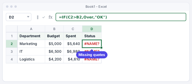
- Text without quotes: in the picture,
Overis missing its quotes, so Excel takes it for a name that doesn't exist. - Function in another language: English Excel doesn't understand
SUMAorBUSCARVfrom a Spanish tutorial; you needSUMandVLOOKUP. - Misspelled function (
VLOKUP) or one that doesn't exist in your version (for example,XLOOKUPin Excel 2016). - Range without a colon:
B2B10instead ofB2:B10.
When you type =SU, Excel shows a list of functions: pick yours with the arrow keys and press Tab. That way you never misspell it.
The correct version, with both text values in quotes.
Find the failing part with Evaluate Formula
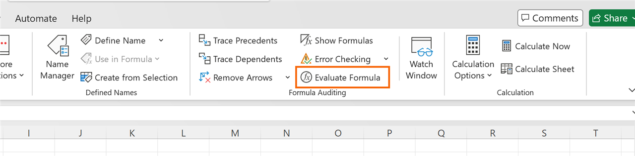
In long formulas it isn't always obvious which piece causes the error. Select the cell and go to Formulas › Formula Auditing › Evaluate Formula. Each time you click Evaluate, Excel calculates the underlined part and shows you the intermediate result, until the error appears and you see exactly where it starts.
In the same group, Trace Precedents draws arrows to the cells the formula uses (clear them with Remove Arrows) and Error Checking walks you through every error on the sheet one by one.
Quick trick: in the formula bar, select part of the formula and press F9 to see its result. Press Esc when you're done so the formula isn't replaced by that value.
Hide only the errors you expect with IFERROR
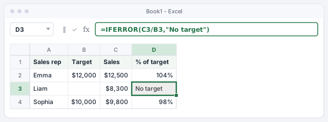
Once you know why an error appears and it's normal for it to appear (a new rep with no target, a code that isn't in the catalog yet), you can replace it with something clearer. IFERROR has two parts: the formula and what to show if it errors: =IFERROR(C2/B2,"No target").
For lookups, IFNA is better: it only hides #N/A and lets any other error, which really is a problem, show through.
Shows No target if the division returns any error.
Hides only the lookup's #N/A.
Don't wrap all your formulas in IFERROR with a 0: you'll hide real errors and a total can come out wrong without anyone noticing.
Expert tips
- See every formula at once. Formulas › Formula Auditing › Show Formulas displays formulas instead of results. It's the fastest way to spot a row that breaks the pattern. Click again to see the values.
- Ask AI for help with context. Paste the formula, the exact error and a couple of sample rows into ChatGPT, and mention your Excel's language and separator. You'll get a formula with the right names. More in asking AI for formulas and checking them.
- Prevent #REF! with tables. Formulas that use Excel tables with references like
Sales[Amount]adapt automatically when you add or remove rows.
Common mistakes and how to fix them
You wrap every formula in IFERROR so the sheet looks clean.
That also hides the real errors, like a deleted reference. Use IFERROR only when you know the cause, and IFNA for lookups.
You see #REF! and type any reference over it.
If you've just deleted something, press Ctrl+Z to get the original reference back. If not, work out which cell the formula should use before rewriting it.
You copy a formula from a Spanish or European site and get #NAME? or a formula error.
Translate the function names (SUMA is SUM, SI is IF, BUSCARV is VLOOKUP) and replace the semicolons between arguments with commas.
You see ##### and think the formula is wrong.
It's not an error: the column is too narrow for the number or date. Double-click the right edge of the column header to widen it.
In Excel for Mac the errors mean the same thing and IFERROR and IFNA work the same way. The auditing tools are also on the Formulas tab; to undo, use ⌘+Z instead of Ctrl+Z.
Frequently asked questions
What is #SPILL!?
It appears with formulas that return several results, such as FILTER or UNIQUE, when the cells where they need to land aren't empty. Clear whatever is below or to the right and the result appears by itself. We explain it in FILTER, SORT and UNIQUE.
What about #NUM! and #NULL!?
#NUM! means an impossible numeric calculation, such as a result that's too large or a function that can't find a solution. #NULL! usually appears when you type a space where a colon or a comma should go between two ranges.
Excel warns me about a circular reference. What is it?
A formula that, directly or indirectly, uses its own cell, for example a total that includes itself. Find it in Formulas › Formula Auditing › Error Checking › Circular References and fix the range.
Why do some formulas online use semicolons?
In much of Europe and Latin America, Excel uses the semicolon to separate arguments and the comma for decimals. Replace each ; with , (and decimal commas with points) and the formula will work in English Excel.
Official sources
Microsoft documentation consulted for this guide.
Saved only in this browser.