VLOOKUP step by step (and its four classic mistakes)
VLOOKUP looks for a value in the first column of a table and returns the item from the column you specify, in the same row. You write =VLOOKUP(A2,Products!$A$2:$D$6,3,FALSE): what to look for, the table (locked with $), the column number and FALSE for an exact match. Forgetting FALSE or the $ signs are the most common mistakes.
It happens when you put together a quote or an order: you type a product code and then go to the price list to copy the name and price, row by row. With twenty products it takes a while; with two hundred, a whole afternoon and a mistake nobody spots until the invoice goes out.
VLOOKUP (the V stands for “vertical”) automates that lookup. It works like the index tabs on a filing cabinet: find the code in the first column, go down to its row and read the box you need by counting columns to the right. It's the most widespread lookup function in Excel and you'll find it in almost every file people send you.
In this guide you write your first VLOOKUP across two sheets and, above all, learn to avoid its four classic mistakes: forgetting FALSE, not locking the table with $, looking up in a column that isn't the first one, and #N/A errors from codes that look the same but aren't.
What you'll learn
- What the four VLOOKUP arguments mean
- How to pull data from another sheet and copy the formula without it shifting
- Why you should always type FALSE at the end
- How to show a clear message instead of #N/A
- When it's worth switching to XLOOKUP
Step by step
Make sure the code is in the first column
The Products sheet holds the price list: Code in column A, Product in B, Price in C and Stock in D, from row 2 to row 6. On the Order sheet you only type the code and the units.
This is the golden rule of VLOOKUP: it only searches the first column of the table you give it and only returns columns to its right. Here the code is in A, so everything fits.
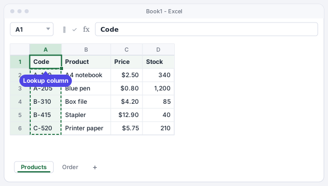
If you need to look up by name to get the code (which is to the left), VLOOKUP can't do it. Use XLOOKUP or INDEX with MATCH.
Understand the four arguments
The structure is VLOOKUP(lookup_value, table_array, col_index_num, range_lookup):
- lookup_value: the order's code,
A2. - table_array: the whole list, starting with the code column:
Products!A2:D6. - col_index_num: which column of that table to read, counting from the first. Product is
2; Price is3. - range_lookup:
FALSEso it looks for the exact code.

Write your first VLOOKUP to bring in the product name
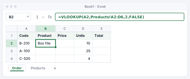
On the Order sheet, click B2 and type =VLOOKUP(. Click A2, type ,, switch to the Products sheet, select A2:D6 and finish the formula:
=VLOOKUP(A2,Products!A2:D6,2,FALSE)
Press Enter: Box file appears, the product with code B-310. The ! separates the sheet name from the cells.
Looks up the code in A2 on the Products sheet and returns column 2 (Product).
If you prefer a wizard with one box per argument, go to Formulas › Function Library › Lookup & Reference and choose VLOOKUP.
Lock the table with F4 before copying the formula
If you copy the formula down as it is, in row 3 the table shifts to Products!A3:D7 and the A4 notebook (which is in row 2) drops out of the search: result, #N/A. That's classic mistake number two.
The fix: in the formula bar, put the cursor on A2:D6 and press F4. Excel adds the $ signs, which mean “this reference doesn't move”:
=VLOOKUP(A2,Products!$A$2:$D$6,2,FALSE)
Now copy it down by double-clicking the small square at the bottom-right corner of the cell. A2 has no $ on purpose, so it becomes A3, A4…
The same lookup with the table locked so you can fill it down.

Change the column number to bring in the price
For the price, the formula is identical except for the third argument: Price is column 3 of the table. In C2:
=VLOOKUP(A2,Products!$A$2:$D$6,3,FALSE)
Fill it down and calculate the total in E2 with =C2*D2. Result: 10 box files at $4.20 make $42.00; 25 notebooks at $2.50, $62.50; 4 packs of paper at $5.75, $23.00.
Returns column 3 (Price) for the product looked up.
Price times units.
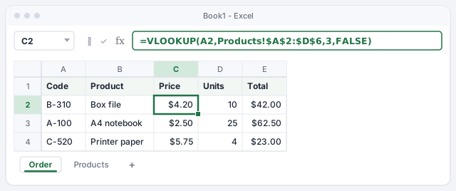
The column number counts within the table you selected, not from column A of the sheet. If your table started in column C, column C would be number 1.
Show a clear message when the code doesn't exist
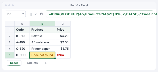
If someone types a code that isn't in the list (for example D-999 in A5), VLOOKUP returns #N/A. Wrap the formula in IFNA, which only steps in for that error:
=IFNA(VLOOKUP(A5,Products!$A$2:$D$6,2,FALSE),"Code not found")
The first argument is your usual VLOOKUP; the second is what to show if it fails. Do the same for the price column (for example with 0 as the second argument) so the total doesn't inherit the error.
Shows “Code not found” instead of #N/A.
IFNA has been around since Excel 2013. Avoid IFERROR for this: it hides every error, even the ones you should see, such as a mistyped table.
Never leave out FALSE: see what happens if you forget it
The fourth argument is optional, and that's the trap: if you don't type it, Excel uses an approximate match. With a code that doesn't exist, such as B-300, it doesn't return an error: it returns the closest value below it in alphabetical order, Blue pen. Wrong data that looks right.
=VLOOKUP(A2,Products!$A$2:$D$6,2) → Blue pen (wrong)
=VLOOKUP(A3,Products!$A$2:$D$6,2,FALSE) → #N/A (correct: that code doesn't exist)
It's classic mistake number one, and the most dangerous because it gives no warning. If the list were also unsorted, the results would be even less predictable.
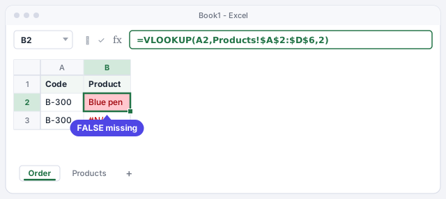
Check any VLOOKUP you inherit from other files or get from AI: if it doesn't end in FALSE (or 0, which is equivalent), fix it.
Expert tips
- Don't let inserted columns break it. The column number is fixed: if someone inserts a column in Products, the
3no longer points at the price. Calculate it withMATCH:=VLOOKUP(A2,Products!$A$2:$D$6,MATCH("Price",Products!$A$1:$D$1,0),FALSE). - #REF! means “that column doesn't exist”. You asked for column 5 of a 4-column table. Widen the table or fix the number.
- Use an Excel table as the source. If you turn the price list into a table (how to create tables), new products join the lookup automatically without touching the ranges.
- If you have Microsoft 365 or Excel 2021, try XLOOKUP. The same lookup without counting columns and with a built-in message:
=XLOOKUP(A2,Products!$A$2:$A$6,Products!$B$2:$B$6,"Code not found"). We explain it in XLOOKUP step by step.
Common mistakes and how to fix them
Mistake 1: it returns data that doesn't match, without showing any error.
FALSE is missing at the end and Excel used an approximate match. Add ,FALSE as the fourth argument.
Mistake 2: the first row works, but #N/A appears when you copy it down.
The table isn't locked and has shifted. Select the range in the formula, press F4 to add the $ signs and copy again.
Mistake 3: #N/A when looking up by a column that isn't the first.
VLOOKUP only searches the first column of the table and only returns columns to its right. Start the table at the lookup column or use XLOOKUP.
Mistake 4: #N/A even though you can see the code in the list.
There are invisible spaces, or the code is a number on one sheet and text on the other. Clean up with =TRIM(A2) and use the same format in both columns.
In Excel for Mac VLOOKUP works the same way, with the same arguments. To lock references with $ use ⌘+T (or F4, depending on your keyboard settings).
Frequently asked questions
When does it make sense to use TRUE or leave the fourth argument empty?
Only for lookups by bands: commission tables, discounts by amount or rate tables, with the first column sorted from smallest to largest. For codes, names or IDs, always use FALSE.
Is VLOOKUP case-sensitive?
No. “a-100” and “A-100” count as the same. What does matter is spaces and whether the data is the same type (number or text).
My Excel rejects the commas. What do I do?
In many European and Latin American countries Excel uses ; as the argument separator. If that's your case, replace the commas between arguments with semicolons.
Should I keep using VLOOKUP or switch to XLOOKUP?
If everyone who uses the file has Microsoft 365 or Excel 2021 or later, XLOOKUP is easier and safer. If someone is on Excel 2019 or earlier, VLOOKUP (or INDEX and MATCH) is still the compatible choice.
Official sources
Microsoft documentation consulted for this guide.
Saved only in this browser.