XLOOKUP: find data in another table in seconds (and forget VLOOKUP)
XLOOKUP looks for a value in one column and returns the item from the same row in another column. You write it like this: =XLOOKUP(B2,Customers!A2:A6,Customers!B2:B6,"Not found"): what you look for, where to look, what to return and what to show if it isn't there. It finds exact matches by default, works to the left and is available in Microsoft 365, Excel 2021 and later.
It happens all the time: one sheet has the orders with the customer ID, and another sheet has the customer list with each name and city. To finish the report you copy names by hand, one by one, or ask whoever “knows how to do VLOOKUP”. And if someone inserts a column in the customer list, everything goes wrong.
XLOOKUP does what you'd do with your finger: find the ID in the customer list, move along that same row and read the name. You tell it what to look for, where to look and which column to read. No counting columns and no remembering to put FALSE at the end.
In this guide you write your first XLOOKUP across two sheets, handle IDs that don't exist, return several columns at once, look up to the left and calculate discounts by amount tiers.
What you'll learn
- The three required arguments of XLOOKUP and the three optional ones
- How to pull data from another sheet and fill the formula down without errors
- How to show a clear message when an ID doesn't exist
- How to return several columns and look up to the left
- How to assign tiered discounts with approximate matching
Step by step
Set up the table you'll look up in
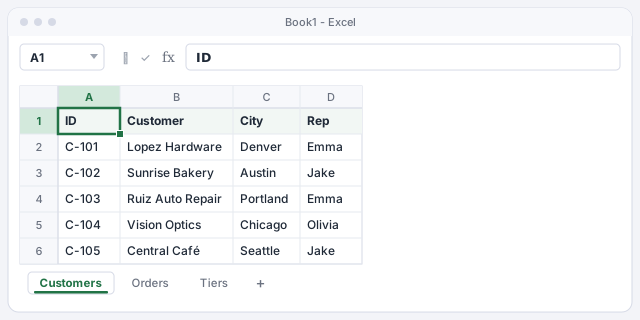
The Customers sheet has one row per customer: ID in column A, Customer in B, City in C and Rep in D. The data runs from row 2 to row 6. On the Orders sheet, each order only carries the customer ID in column B.
The only requirement is that each ID appears just once in the customer list. If there are duplicates, XLOOKUP returns the first one it finds.
IDs must be typed the same way on both sheets: “C-103” is not the same as “C-103 ” with a trailing space.
Understand the three required arguments
The full structure is:
XLOOKUP(lookup_value, lookup_array, return_array, [if_not_found], [match_mode], [search_mode])
- lookup_value: the order's ID,
B2. - lookup_array: the ID column on the Customers sheet,
Customers!$A$2:$A$6. - return_array: the column you want to read,
Customers!$B$2:$B$6.
The last three, in brackets, are optional. The ! sign separates the sheet name from the cells.

lookup_array and return_array must have the same number of rows. Otherwise the formula returns #VALUE!.
Write your first XLOOKUP on the Orders sheet
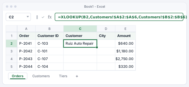
Go to the Orders sheet, click C2 and type =XLOOKUP(. Click B2, type ,, switch to the Customers sheet and select A2:A6; press F4 to lock it with $. Type ,, select B2:B6, press F4 and close the parenthesis:
=XLOOKUP(B2,Customers!$A$2:$A$6,Customers!$B$2:$B$6)
Press Enter: Ruiz Auto Repair appears, customer C-103. If you prefer a wizard, the function is under Formulas › Function Library › Lookup & Reference.
Looks up the ID in B2 on the Customers sheet and returns the customer name.
Add a message for IDs that don't exist
If an ID isn't in the list, XLOOKUP returns the #N/A error (“not available”). That's correct, but it looks bad and worries whoever reads the report. Add the fourth argument with the text you want to show:
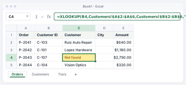
=XLOOKUP(B2,Customers!$A$2:$A$6,Customers!$B$2:$B$6,"Not found")
Fill the formula down by double-clicking the small square at the bottom-right corner of C2. Order P-2043 has ID C-107, which doesn't exist: it now shows Not found and you know exactly what to check.
Same as before, but shows “Not found” instead of #N/A.
Thanks to the $ signs you added with F4, the lookup column stays put when you copy; only B2 changes to B3, B4, B5.
Return several columns with a single formula
Want the city too? You don't need another formula. For return_array, select two columns, B2:C6:
=XLOOKUP(B2,Customers!$A$2:$A$6,Customers!$B$2:$C$6,"Not found")
The result spills: the name appears in C2 and the city in D2, even though the formula is only in C2. Fill down as before. Spilling means one formula fills several neighboring cells by itself.
Returns the customer's name and city at once (spills into D2).
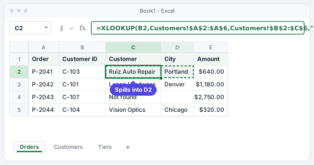
If the cell next to it (D2) has anything in it, you'll see #SPILL!. Clear those cells and the result appears.
Look up to the left without rearranging anything
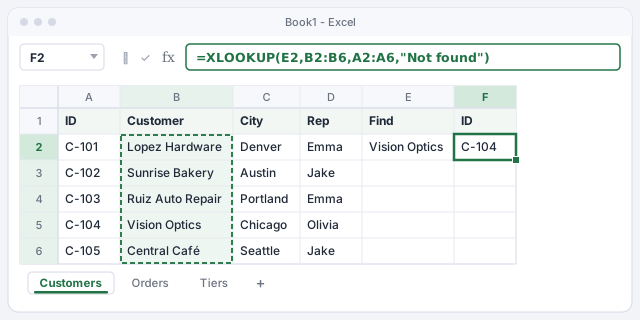
With VLOOKUP the lookup column has to be the first column of the table. With XLOOKUP it doesn't matter. On the Customers sheet, type a name in E2 and get its ID (which sits to the left) in F2:
=XLOOKUP(E2,B2:B6,A2:A6,"Not found") → C-104
No sheet names are needed here because everything is on the same sheet.
Looks up the name in E2 in the Customer column and returns the ID to its left.
Calculate tiered discounts with approximate matching
The Tiers sheet holds the minimum amount for each tier and its discount:
| From (A) | Discount (B) |
|---|---|
| 0 | 0% |
| 500 | 2% |
| 1,000 | 5% |
| 2,500 | 8% |
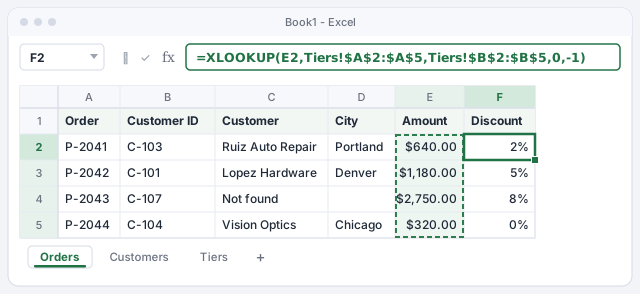
A $1,180 order isn't in the list, but it should get 5%. The fifth argument, match_mode, solves it: -1 means “exact match or, if there isn't one, the next smaller item”. In F2 on Orders:
=XLOOKUP(E2,Tiers!$A$2:$A$5,Tiers!$B$2:$B$5,0,-1)
Results: $640 → 2%, $1,180 → 5%, $2,750 → 8%, $320 → 0%. The 0 in the fourth argument is what it returns if an amount doesn't reach any tier.
Looks up the amount in the tier table and returns the discount of the nearest lower tier.
match_mode 1 does the opposite: it finds the next larger item. Handy for rates like “up to 5 lb”.
Expert tips
- Tables read better. Turn the list into a table named Customers (Ctrl+T) and write
=XLOOKUP(B2,Customers[ID],Customers[Customer],"Not found"). New customers are picked up automatically and you don't need $. More in Excel tables. - The last match, not the first. A sixth argument of
-1searches from the bottom up. On the Orders sheet,=XLOOKUP("C-101",B2:B5,A2:A5,"No orders",0,-1)returns that customer's most recent order. - Match part of the text. With match_mode
2you can use wildcards:=XLOOKUP("*Sun*",Customers!B2:B6,Customers!A2:A6,"Not found",2)returns C-102 (Sunrise Bakery). - Ask AI for it, then test it. Tell ChatGPT or Copilot: “write an XLOOKUP that looks up B2 in Customers!A2:A6 and returns Customers!B2:B6”. Then test it with one ID that exists and one that doesn't.
Common mistakes and how to fix them
You get #N/A even though the ID is in the list.
It's almost always invisible spaces or a number stored as text on one of the sheets (101 versus “101”). Clean up with =TRIM(B2) and make sure both columns hold the same type of data.
You get #NAME? when the file is opened on another computer.
That Excel is 2019 or earlier and doesn't have XLOOKUP. Use VLOOKUP or INDEX with MATCH, which work in every version.
You get #SPILL! when returning several columns.
The cells the result needs to spill into aren't empty. Clear them or move the formula to a free area.
When you fill the formula down, the results shift or show #N/A.
The ranges on the Customers sheet are missing their $ signs. Select each range in the formula bar and press F4, or use a table.
XLOOKUP is available in Excel for Mac with Microsoft 365 or Excel 2021 and later, with the same arguments. To lock references with $ use ⌘+T (or F4, depending on your keyboard settings).
Frequently asked questions
Why is XLOOKUP better than VLOOKUP?
It finds exact matches by default, can return columns to the left, doesn't break when you insert columns (it doesn't count positions), returns several columns at once and has its own “not found” argument. If you still need VLOOKUP, see VLOOKUP step by step.
Which versions of Excel have XLOOKUP?
Microsoft 365, Excel 2021, Excel 2024 and Excel for the web. If you share the file with someone on Excel 2019 or earlier, use INDEX and MATCH.
My Excel rejects the commas. What do I do?
In many European and Latin American countries Excel uses ; as the argument separator. If that's your case, replace the commas between arguments with semicolons.
Is XLOOKUP case-sensitive?
No. “ruiz auto repair” and “Ruiz Auto Repair” count as the same. Spaces and accents do matter.
Official sources
Microsoft documentation consulted for this guide.
Saved only in this browser.