INDEX and MATCH: flexible lookups that work in any version of Excel
MATCH tells you the position of a value in a list, and INDEX returns the value at that position in another column. Together they make a flexible lookup: =INDEX(C2:C6,MATCH(E2,A2:A6,0)) finds the code in E2 within A2:A6 and returns its price from C2:C6. The final 0 is required for an exact match.
It happens with VLOOKUP: the column you need sits to the left of the one you search, and there's no way around it. Or someone inserts a column in the table and all your formulas start returning the wrong data. And if you share the file with someone on an older Excel, XLOOKUP isn't an option either.
The INDEX + MATCH combo solves all of that and works in every version of Excel. Think of a parking garage: MATCH is the attendant who tells you “your car is in spot 3”, and INDEX is the valet who goes to spot 3 in whichever row you name and brings back what's there. On their own they look modest; together they look up in any direction.
In this guide you learn each one separately, combine them with a real product catalog, and finish with a lookup by row and column at the same time, like in a quarterly sales table.
What you'll learn
- What MATCH does and why its third argument should be 0
- What INDEX does and how to plug MATCH into it
- How to look up to the left, which VLOOKUP can't do
- How to look up by row and column at once in a two-way table
- How to show a clear message when the value doesn't exist
Step by step
Find the position of a value with MATCH
You have a catalog with codes in A2:A6, products in B2:B6 and prices in C2:C6. In E2 type the code you're looking for (P-103) and in F2 type =MATCH(E2,A2:A6,0).
The result is 3: P-103 is the third item in the range A2:A6. Note that it doesn't return the sheet row (row 4) but the position inside the range. The three arguments are: what you look for, where you look for it, and the match type (0 = exact).
Returns the position of the code in E2 within A2:A6.
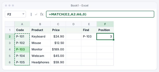
If you leave out the last argument, MATCH uses 1 (approximate match) and, on an unsorted list, returns wrong positions without any warning. Always type the 0.
Get the value at a position with INDEX
Now the other half. INDEX takes a range and a row number and returns whatever is at that position. Type 3 in E2 and in F2 type =INDEX(C2:C6,E2). The result is $189.00, the third price in the list.
As before, the number is the position inside the range, not the sheet row. Change E2 to 5 and you get $59.90.
Returns the value at position E2 within C2:C6.
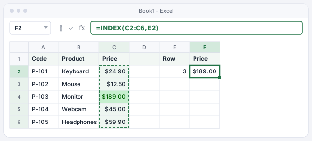
Combine them: MATCH inside INDEX
Instead of typing the position by hand, let MATCH work it out. Type P-103 in E2 again and in F2 type =INDEX(C2:C6,MATCH(E2,A2:A6,0)).
Read it from the inside out: MATCH finds P-103 among the codes and returns 3; INDEX goes to position 3 of the prices and returns $189.00. Change the code in E2 and the price updates by itself.
Finds the code in E2 and returns its price.
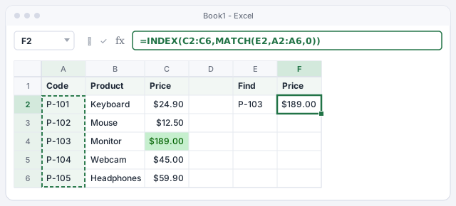
Both ranges must be the same size and start on the same row (A2:A6 and C2:C6). If one starts on row 1 and the other on row 2, the result is shifted by one row.
Look up to the left
Here's the edge over VLOOKUP: the column you return can be on either side. Type Webcam in E2 and in F2 type =INDEX(A2:A6,MATCH(E2,B2:B6,0)).
You search the Product column (B) and return the Code column (A), which sits to its left. Result: P-104. And because there's no hard-coded column number, inserting or moving columns in the catalog doesn't break the formula.
Searches the product name and returns the code, which is to the left.

Lock the ranges with $ and copy the formula down
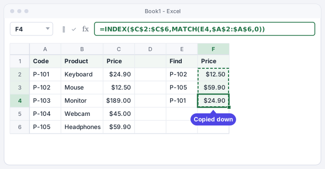
If you're going to look up several codes, lock the ranges so they don't move when you drag. Type the formula in F2 with absolute ranges: =INDEX($C$2:$C$6,MATCH(E2,$A$2:$A$6,0)). To add the $ signs, click inside the range in the formula bar and press F4.
Drag the fill handle (the small square at the corner of F2) down to F4. Only E2 changes, becoming E3 and E4; the ranges stay put. We cover this in depth in relative and absolute references.
Ranges locked with $; only E2 changes as you copy down.
Look up by row and column at the same time
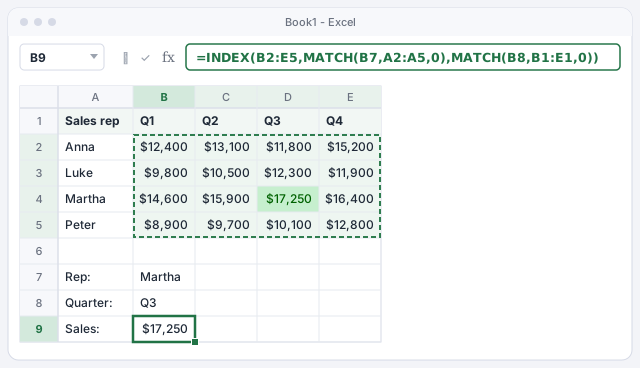
INDEX accepts a third argument: the column number. Give it two MATCH functions, one for the row and one for the column, and you can search a two-way table. In this quarterly sales table, type the rep in B7, the quarter in B8 and, in B9:
=INDEX(B2:E5,MATCH(B7,A2:A5,0),MATCH(B8,B1:E1,0))
The first MATCH finds Martha at position 3 of the names; the second finds Q3 at position 3 of the headers. INDEX returns the intersection: $17,250.
Crosses the rep in B7 with the quarter in B8.
Turn B7 and B8 into drop-down lists and you'll have a lookup tool nobody can break by misspelling a name.
Show a clear message when the value doesn't exist
If you look up a code that isn't in the list, MATCH returns #N/A and the error flows into INDEX. Wrap the formula in IFERROR to show readable text instead:
=IFERROR(INDEX(C2:C6,MATCH(E2,A2:A6,0)),"Not found")
With P-999 in E2, the cell shows Not found instead of the error. If the code does exist, you see the price as usual.
If the code doesn't exist, shows “Not found” instead of #N/A.

IFERROR hides every error, including those from a mistyped formula. To catch only “not found”, use =IFNA(INDEX(C2:C6,MATCH(E2,A2:A6,0)),"Not found") (Excel 2013 or later).
Expert tips
- Look up with two conditions. Multiply the comparisons and match the 1:
=INDEX(D2:D20,MATCH(1,(A2:A20=G1)*(B2:B20=G2),0))returns the value from the row where column A equalsG1and column B equalsG2. In Excel 2019 or earlier, confirm it with Ctrl+Shift+Enter. - Use it with Excel tables. With a table named
Products, the formula reads itself and grows with the data:=INDEX(Products[Price],MATCH(E2,Products[Code],0)). More in Excel tables. - On Microsoft 365 or Excel 2021?
XLOOKUPdoes the same in one function, andXMATCHis aMATCHthat defaults to exact. INDEX and MATCH remain the safe choice if people with older versions open the file. See XLOOKUP step by step. - Ask AI for it, then test it. ChatGPT writes these formulas well, but check that the ranges start on the same row and test with two or three codes whose answer you know by heart.
Common mistakes and how to fix them
The formula returns a value from a different row, with no error.
The 0 at the end of MATCH is missing, or the two ranges don't start on the same row. Make sure it reads =MATCH(E2,A2:A6,0) and that the INDEX range runs from row 2 to row 6, like the lookup range.
You get #N/A even though the code is in the list.
There are usually extra spaces or numbers stored as text. Check for hidden spaces with =LEN(A4), clean them with TRIM, or convert the text to numbers.
When you copy the formula down, results turn into #N/A after a certain row.
The ranges have shifted. Lock them with $ (press F4 inside the range) so they read $A$2:$A$6 and $C$2:$C$6.
In Excel for Mac the formulas are identical. To lock references with $ you can use ⌘+T or Fn+F4, depending on your keyboard settings.
Frequently asked questions
Is INDEX and MATCH better than XLOOKUP?
If everyone uses Microsoft 365 or Excel 2021 or later, XLOOKUP is shorter and easier to read. If the file will be opened in older versions, INDEX and MATCH work in all of them.
Why do people say it beats VLOOKUP?
Because it looks up to the left, doesn't rely on a hard-coded column number that breaks when you insert columns, and can search by row and column at once. If you still use VLOOKUP, review its four classic errors.
Can I look up data on another sheet?
Yes. Include the sheet name in the ranges: =INDEX(Products!C2:C6,MATCH(E2,Products!A2:A6,0)). The easiest way is to start typing the formula and select the ranges with the mouse on the other sheet.
Does it matter whether my lookup column is sorted?
Not with match type 0: an exact match works on any order. Sorting only matters if you use 1 or -1 for approximate matches, such as finding a tax bracket or a discount tier.
Official sources
Microsoft documentation consulted for this guide.
Saved only in this browser.