Relative and absolute references ($A$1): why your formula breaks when you drag it
When you drag a formula, Excel shifts its references (they are relative). To stop a cell from moving, make it absolute with the $ sign: =B2*$E$2. The quick way: edit the formula, put the cursor on the reference and press F4, which cycles through $E$2, E$2, $E2 and E2. On a Mac, ⌘+T.
It happens every time: you work out the sales tax for the first product, the formula works, you drag it down… and every other row shows zero. Or worse, #VALUE!. You didn't type anything wrong: Excel did exactly what it does by default, which is shift references when you copy.
Think of references as directions. A relative reference (E2) is like saying “the house next door”: it depends on where you're standing. An absolute reference ($E$2) is a street address: you end up in the same place wherever you start. The $ sign is the anchor.
In this guide you'll see why the formula breaks, how to fix it in one second with F4, and how to use mixed references to fill a whole table with a single formula.
What you'll learn
- Why a formula works in the first row and fails when you drag it
- How to lock a cell with $ using the F4 key
- The difference between relative, absolute and mixed references
- How to fill a two-way table with a single formula
- How to use a name instead of $ so the formula reads better
Step by step
Type the formula and drag it down
You have a list of products with their price in column B and the sales tax rate (8%) in cell E2. In C2 you type =B2*E2 and get $2.00. Perfect.
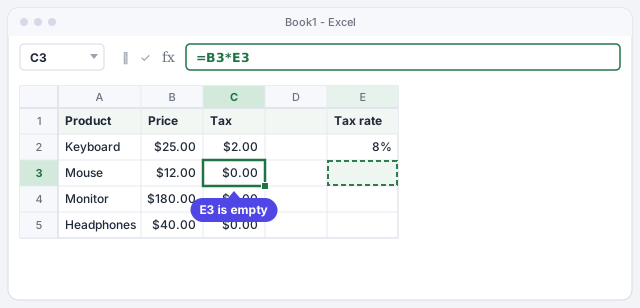
Now you drag the fill handle (the small square at the bottom-right corner of the cell) down to C5. Result: every new row shows $0.00.
Starting formula: it works in C2 but breaks when copied down.
Your tax rate may be different (VAT, GST, state sales tax…). The method is identical: just change the value in E2.
Look at what Excel did to your formula
Click C3 and look at the formula bar: it says =B3*E3. Excel moved both references down one row. For B that's exactly what you wanted (the mouse price), but the tax rate isn't in E3: that cell is empty, so it counts as zero.
That's a relative reference: Excel doesn't store “cell E2”, it stores “the cell two columns to the right, in this same row”. When you copy, the directions stay the same and the destination changes.

To see every formula at once instead of its result, go to Formulas › Formula Auditing › Show Formulas. Click it again to go back.
Lock the tax cell with the F4 key
Select C2 and press F2 to edit it (or click in the formula bar). Put the cursor on E2 inside the formula and press F4. The reference becomes $E$2. Press Enter.
A $ before the letter locks the column; a $ before the number locks the row. With both, the cell never moves. You can also type the $ yourself (Shift+4 on a US keyboard).
B2 stays relative (moves down with each row); $E$2 is anchored.

On many laptops F4 controls brightness or volume. If nothing happens, try Fn+F4.
Copy the formula all the way down again
With C2 selected, double-click the fill handle. Excel copies the formula down to the last row with data in the column next to it. Now C5 contains =B5*$E$2 and every amount is right.
Always check the last row: if its formula points where it should, the ones in between do too.

Learn the four reference types
Each time you press F4 on a reference, Excel switches to the next type and, after the fourth, starts over:
| Reference | Type | When copied… |
|---|---|---|
E2 | Relative | row and column both move |
$E$2 | Absolute | nothing moves |
E$2 | Mixed | row 2 is locked; the column moves |
$E2 | Mixed | column E is locked; the row moves |
A rule to remember it: the $ anchors whatever comes right after it.

Fill a two-way table with a mixed reference
Mixed references shine in tables with inputs in a row and a column. Here you have prices in column A and discounts in row 1. In B2 type =$A2*(1-B$1) and copy the cell to the whole range B2:D4.
$A2 means “always column A, whatever row” and B$1 means “always row 1, whatever column”. One formula fills all nine cells: for example, D4 works out 80 × (1 − 20%) = 64.
Copy it to B2:D4: each cell takes its price from column A and its discount from row 1.

Alternative: give the fixed cell a name
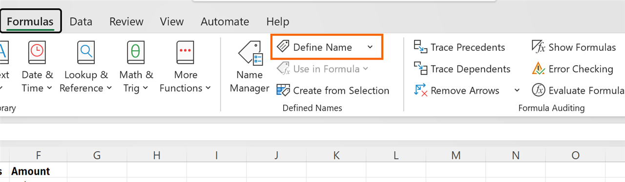
Select E2, click the Name Box (left of the formula bar, where it says E2), type TaxRate and press Enter. You can also do it from Formulas › Defined Names › Define Name.
From then on you can write =B2*TaxRate. A name behaves like an absolute reference and, on top of that, the formula makes sense when you read it.
Same as =B2*$E$2 once E2 is named TaxRate.
Expert tips
- F4 locks whole ranges too. If you select
B2:B5inside the formula and press F4, it becomes$B$2:$B$5in one go. Perfect for percentage of total:=B2/SUM($B$2:$B$5). - Moving isn't copying. If you cut and paste a formula, or drag the cell border, Excel doesn't change its references. It only adjusts them when you copy or fill.
- In Excel tables you rarely need $. References to table columns copy correctly on their own. We cover it in Excel tables.
- Check formulas the AI gives you. ChatGPT usually gets the logic right but forgets a
$. Drag the formula and check the last row by hand before trusting it. More in asking AI for formulas and checking them.
Common mistakes and how to fix them
You press F4 and the reference doesn't change (or Excel repeats some other action).
F4 only toggles the $ while you're editing the formula. Press F2 or click in the formula bar, put the cursor on the reference, then press F4. Outside edit mode, F4 repeats your last action.
You put $ on every reference and every row gives the same result.
Lock only what must not move. In =B2*$E$2 the price B2 has to move down with each row; if you write $B$2*$E$2, every row calculates the tax of the first product.
After dragging, the new rows show zeros or #VALUE!.
A relative reference shifted to an empty cell (gives zero) or to text (gives #VALUE!). Click the last cell, read its formula and add the $ where it's missing.
In Excel for Mac the $ sign works exactly the same. To cycle through reference types use ⌘+T (on some keyboards F4 also works, sometimes together with the Fn key).
Frequently asked questions
Does the $ sign have anything to do with dollars?
No. Inside a reference, $ only means “don't move this when copying”. It doesn't change the cell's currency format or the result.
Does the same thing happen when I copy the formula to the right?
Yes. Copying down changes row numbers; copying across changes column letters. That's why sometimes you only need to lock one of them (a mixed reference).
Is it better to use $E$2 or a name like TaxRate?
They work the same. The name reads better and doesn't break if you move the value with cut and paste. To dig deeper, see Defined names and LET.
How do I copy the formula without dragging?
Copy the cell with Ctrl+C, select the destination range and paste with Ctrl+V. References adjust just as they do when dragging. More methods in fill handle and Flash Fill.
Official sources
Microsoft documentation consulted for this guide.
Saved only in this browser.