Your first formulas: SUM, AVERAGE, MAX, MIN and AutoSum
Every Excel formula starts with =. To add up a range type =SUM(B2:B7); for the mean, =AVERAGE(B2:B7); for the highest and lowest values, =MAX(B2:B7) and =MIN(B2:B7). Without typing anything: select the cell below the numbers and click Home › Editing › AutoSum; the button's arrow also offers Average, Max and Min.
It happens every time: you have a column of amounts and you grab the calculator on your phone to add them up. Then a number changes and you start over. Or you type the total into the cell by hand and, three weeks later, nobody knows where it came from.
A formula is an instruction you give Excel so it does the math for you, and it recalculates by itself when the data changes. It's like writing down the sum instead of just the answer: if one number changes, the total changes too. A function (SUM, AVERAGE…) is a ready-made formula: you only tell it which cells to work with.
In this guide you'll write your first four functions on real monthly sales and learn to use AutoSum, the button that writes them for you.
What you'll learn
- How to write a formula and read it in the formula bar
- What a range is and how to write it (B2:B7)
- When to use SUM, AVERAGE, MAX and MIN
- How to use AutoSum and its menu so you don't type anything
- Why you should never type a total by hand
Step by step
Start the formula with an equals sign
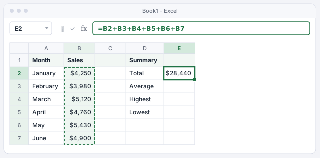
You have January to June sales in B2:B7. Click E2, type =, then click B2, type +, click B3, and so on down to B7. Press Enter: the cell shows $28,440.
Notice the difference: the cell shows the result and the formula bar (above the columns) shows the formula. Without the leading =, Excel would treat it as text and calculate nothing.
It works, but with 200 rows it would take forever: we shorten it in the next step.
Replace the long sum with the SUM function
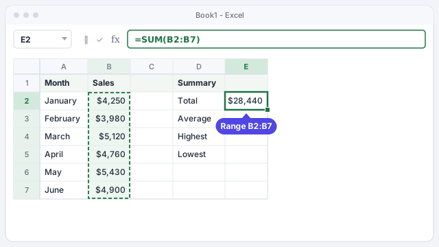
In E2 type =SUM(, select cells B2 to B7 with the mouse, close the parenthesis and press Enter. Same result, much shorter formula: =SUM(B2:B7).
B2:B7 is a range: a group of cells from the first to the last. Read the colon as “through”. While you type =SU, Excel suggests functions in a list; pick one with the arrow keys and press Tab to accept it.
Adds every cell from B2 to B7: $28,440.
SUM accepts several ranges separated by commas: =SUM(B2:B7,D2:D7) adds both columns at once.
Get the mean with AVERAGE
In E3 type =AVERAGE(B2:B7) and press Enter. Result: $4,740, which is 28,440 / 6. That's average sales per month.
AVERAGE adds up the range and divides by the number of cells that contain numbers. Empty cells and text don't count, but a 0 does: if a month had no sales, decide whether you type 0 or leave it blank, because the result changes.
Mean of the six months: $4,740.

Find the best and worst month with MAX and MIN
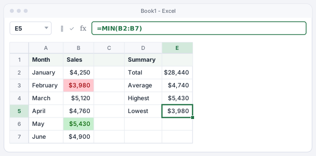
In E4 type =MAX(B2:B7) and in E5, =MIN(B2:B7). You get $5,430 (May) and $3,980 (February).
With six rows you can spot it by eye; with six hundred, you can't. MAX and MIN work just as well for the most expensive invoice, the lowest grade or the most recent date in a list (to Excel, dates are numbers too).
Highest value in the range: $5,430.
Lowest value in the range: $3,980.
Let AutoSum write the formula for you
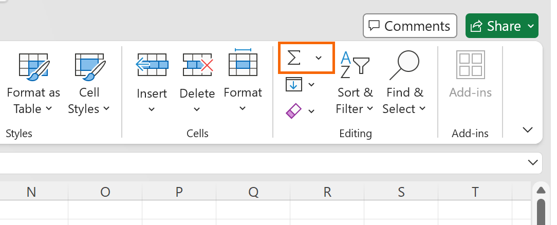
Click the cell right below the numbers (B8) and go to Home › Editing › AutoSum (it's also in Formulas › Function Library › AutoSum). Excel types =SUM(B2:B7) and puts a dashed border around the range it guessed.
If the range is right, press Enter. If not, select the correct range with the mouse before pressing Enter. The keyboard shortcut is Alt+=.
What AutoSum types below the sales column.
AutoSum stops at the first empty cell it finds going up. If there's a gap in the column, it only adds the part below it: always check the dashed border.
Pick Average, Max or Min from the AutoSum arrow
The AutoSum button has an arrow on its right. Click it to see Sum, Average, Count Numbers, Max and Min. They all work the same way: select the result cell, pick the function, check the range and press Enter.
Count Numbers writes the COUNT function, which tells you how many cells in the range contain numbers (here, 6).

Change a value and watch everything recalculate
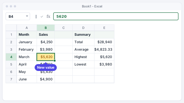
Correct March sales: type 5620 in B4 and press Enter. Without touching anything else, the total becomes $28,940, the average $4,823.33 and the highest $5,620, because March is now the best month.
That's the big advantage of formulas over a total typed by hand: the result is always up to date.
Expert tips
- Check the status bar. Select a range and, at the bottom right, Excel shows Average, Count and Sum without any formula. Right-click the status bar to add Minimum and Maximum too.
- Row and column totals at once. Select the data plus an empty row below and an empty column to the right, then click AutoSum: Excel fills in every total in one go.
- Copy the formula instead of retyping it. If you have a sales column for each rep, write the total under the first one and drag it to the right. We explain how in fill handle and Flash Fill.
- Use AI as a second opinion. If you ask ChatGPT for a formula, compare its result with what the status bar shows for that range. If they don't match, something's wrong.
Common mistakes and how to fix them
SUM returns less than expected and some numbers are left-aligned with a green triangle.
Those numbers are stored as text and SUM ignores them. Select them, click the warning icon that appears next to them and choose Convert to Number.
Excel warns about a circular reference and the total shows 0.
You included the total cell inside the range you're adding, for example =SUM(B2:B8) typed in B8. Fix the range so it ends on the row above: =SUM(B2:B7).
The cell shows the text of the formula instead of the result.
The = sign is missing at the start, there's a space before the =, or the cell was formatted as Text. Set the format to General (Home › Number), retype the formula and press Enter.
In Excel for Mac, AutoSum is on the same tabs (Home and Formulas) and its shortcut is ⌘+Shift+T. SUM, AVERAGE, MAX and MIN are written exactly the same way.
Frequently asked questions
I've seen formulas with semicolons online. Do I need them?
Not in English-language Excel with US regional settings: arguments are separated by commas, as in =SUM(B2:B7,D2:D7). Semicolons appear in Excel set up for regions that use a comma as the decimal separator, such as much of Europe and Latin America.
Can I add up cells that aren't next to each other?
Yes. Separate them with commas: =SUM(B2,B4,B6). You can also hold Ctrl while clicking each cell as you build the formula.
Does AVERAGE count empty cells?
No. It ignores empty cells and cells with text, but it does count zeros. If a month with no sales should pull the average down, type 0; if it shouldn't count, leave it blank.
What if I only want to add up sales for one region or one rep?
That's what conditional functions are for. See SUMIFS and COUNTIFS.
Official sources
Microsoft documentation consulted for this guide.
Saved only in this browser.