SUMIFS and COUNTIFS: sum and count with conditions
SUMIFS adds up only the rows that meet all your conditions. The range you want to sum comes first, followed by pairs of criteria range and criterion: =SUMIFS(D2:D9,B2:B9,"North",C2:C9,"Emma"). COUNTIFS works the same way but has no sum range: it counts the rows. Both are under Formulas › Insert Function, or you can type them straight into the cell.
It happens every month: you have a sales list and someone asks “how much did Emma sell in the North region in September?”. You filter, select, glance at the status bar, jot the number on a sticky note… and the next day they want the same thing for Jake. Every answer costs you five minutes and a little fear of having got it wrong.
SUMIFS is that same question written as a formula. Think of it as a sieve with several screens: each condition is a screen, and only the rows that get through all of them make it to the bottom. Whatever gets through is added up. Its sibling COUNTIFS uses the same sieve, but instead of adding amounts it counts how many rows got through.
In this guide you write both with real sample data, learn to use dates, minimum amounts and cells as criteria, and build a small summary by region that updates itself when you add new sales.
What you'll learn
- The argument order of SUMIFS (and why it differs from SUMIF)
- How to combine several conditions: text, numbers and date ranges
- How to use a cell as the criterion to build a summary you can fill down
- How to count rows with COUNTIFS
- How to double-check the result in ten seconds
Step by step
Lay out your data in columns with headers
Each row is a sale and each column is one piece of information: Date, Region, Rep and Amount. No blank rows in the middle and no merged cells. In the example, the data sits in A1:D9: row 1 holds the headers and the sales run from row 2 to row 9.
A range is a group of cells, for example D2:D9 (the amounts). The formulas in this guide work with whole data columns, always of the same size.
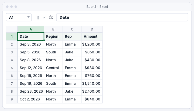
Make sure the amounts are real numbers: if they're left-aligned, they're probably text and the sum will ignore them.
Learn the order: what you sum first, then the conditions
The structure never changes:
SUMIFS(sum_range, criteria_range1, criteria1, criteria_range2, criteria2, …)
- sum_range: the column with the numbers you want to add up (
D2:D9). - criteria_range1: the column where Excel checks the first condition (
B2:B9). - criteria1: what it must match (
"North").
After that, add as many range + criterion pairs as you need. Each pair is one more screen in the sieve.

In SUMIF (without the S) the range to sum goes last. If you mix up the two functions, you'll get nonsense results with no error to warn you.
Write your first formula with one condition
Click cell F2, type the formula and press Enter:
=SUMIFS(D2:D9,B2:B9,"North")
Result: $5,130.00, the total of the five sales in the North region (1,200 + 430 + 760 + 2,100 + 640). Text criteria always go in double quotes.
Adds up the amounts of the rows whose region is North.
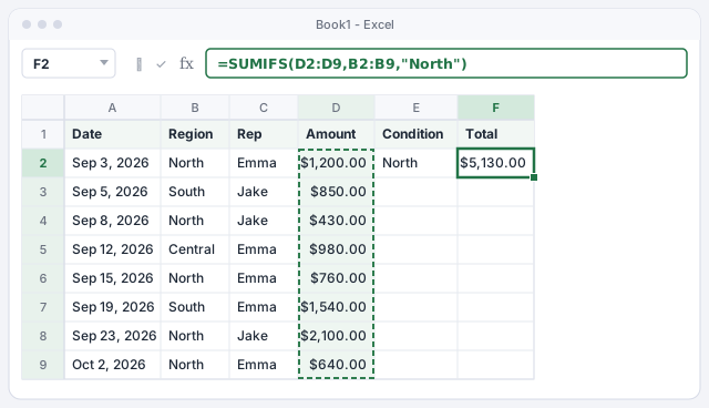
While you type, Excel shows the argument list under the cell and puts the current one in bold. It's the quickest way not to get lost.
Add a second condition
Now the full question: sales by Emma in the North region. Just add another pair at the end:
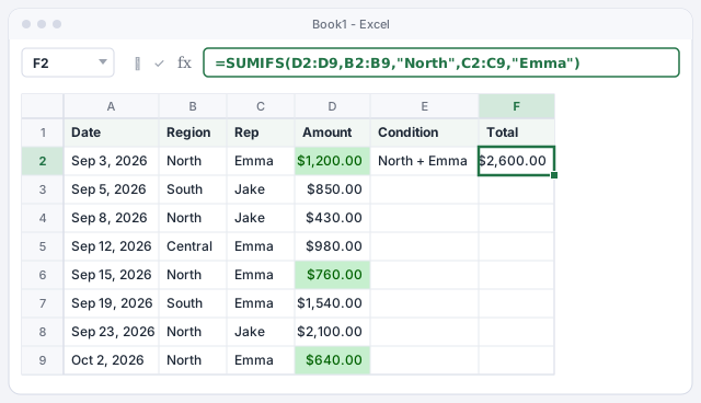
=SUMIFS(D2:D9,B2:B9,"North",C2:C9,"Emma")
Result: $2,600.00 (1,200 + 760 + 640). A row only counts if it meets all the conditions at once: Jake's North sales and Emma's South sale are left out.
Adds up the amounts of the rows that are in the North region and belong to Emma.
Use a cell as the criterion and build a summary by region
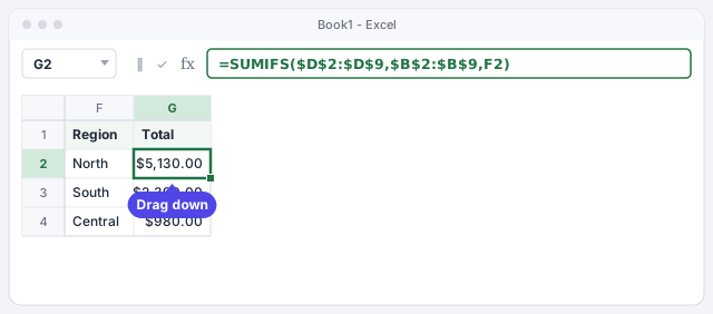
Typing "North" inside the formula is fine for a quick question, but for a report it's better to keep the criterion in a cell. Type the regions in F2:F4 and, in G2:
=SUMIFS($D$2:$D$9,$B$2:$B$9,F2)
The $ signs lock the data ranges so they don't shift when you copy (press F4 with the cursor on the reference to add them). Drag G2 down: South gives $2,390.00 and Central $980.00. If you change an amount tomorrow, the summary updates itself.
Adds up the amounts for the region typed in F2; fill it down for the other regions.
If you turn the data into a table named Sales, the formula reads almost like a sentence: =SUMIFS(Sales[Amount],Sales[Region],F2). And new sales are picked up automatically.
Filter by amounts and dates with operators
For numbers and dates, the criterion includes an operator (>, <, >=, <=, <>) inside the quotes. Sales of $1,000 or more:
=SUMIFS(D2:D9,D2:D9,">=1000") → $4,840.00
Notice that the range you sum and the range you test can be the same. For a period, use two conditions on the date column and join the operator to the date with &. Emma's North sales in September only:
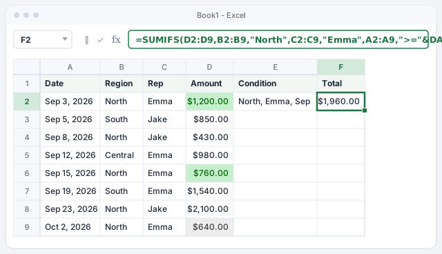
=SUMIFS(D2:D9,B2:B9,"North",C2:C9,"Emma",A2:A9,">="&DATE(2026,9,1),A2:A9,"<="&DATE(2026,9,30)) → $1,960.00
The Oct 2 sale ($640) is left out. DATE(2026,9,1) avoids any confusion between date formats in different countries.
Adds up only the sales of $1,000 or more.
Adds up Emma's North sales between September 1 and September 30, 2026.
Don't type the date as text inside the criterion (">=9/1/2026"): depending on regional settings, Excel may read it as January 9.
Count rows with COUNTIFS
To find out how many sales meet the conditions, use COUNTIFS. It's the same idea without a sum range: it starts straight away with the range + criterion pairs.
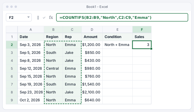
=COUNTIFS(B2:B9,"North",C2:C9,"Emma") → 3 sales by Emma in the North.
=COUNTIFS(D2:D9,">=1000") → 3 sales of $1,000 or more.
Divide the sum by the count and you get the average sale; there's also AVERAGEIFS for that, written exactly like SUMIFS.
Counts the rows in the North region that belong to Emma.
Counts the sales of $1,000 or more.
Double-check the result with a filter
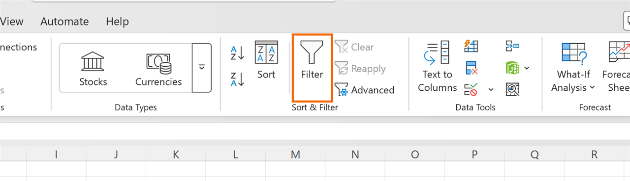
Before you send the report, check it once. Click inside the data and go to Data › Sort & Filter › Filter (or press Ctrl+Shift+L). Filter Region = North and Rep = Emma, select the visible amounts and look at the status bar at the bottom right: it should say Sum: $2,600.00, the same as your formula.
If it doesn't match, it's almost always an extra space in a name or an amount stored as text.
If you ask ChatGPT or Copilot for the formula, always run this check on one case: AI gets the structure right most of the time, but it can swap the argument order or use semicolons where your Excel expects commas.
Expert tips
- Wildcards for partial text. The asterisk stands for any text:
"*Boston*"matches “Boston Downtown Office”. The question mark stands for a single character. - “Not equal to” and “not blank”.
"<>South"sums everything except South;"<>"sums only the rows whose criteria column isn't empty. - Operator plus cell. If the minimum amount is in
H1, write">="&H1: you change the threshold without touching the formula. - For “OR” conditions, add two formulas. North or South:
=SUMIFS(D2:D9,B2:B9,"North")+SUMIFS(D2:D9,B2:B9,"South")gives $7,520.00. If you need lots of combinations, a PivotTable will be easier. - Siblings with the same structure.
AVERAGEIFS,MAXIFSandMINIFS(the last two since Excel 2019) are written the same way: first the range you calculate, then the pairs.
Common mistakes and how to fix them
The formula returns #VALUE!.
The ranges aren't the same size (for example D2:D9 and B2:B10). Every range in the formula must start and end on the same rows.
The result is 0 even though you can see matching rows.
Look for extra spaces ("North " isn't "North") or amounts stored as text. Clean the spaces with =TRIM(B2) and convert the text to numbers.
Excel won't accept the formula when you type a criterion like >=1000.
Criteria with an operator go in quotes: ">=1000". If you use a cell, join the operator with &: ">="&H1.
You fill the formula down and the totals come out wrong.
The data ranges shifted as you copied. Lock them with $ (press F4 on each range) or use a table with structured references.
In Excel for Mac the functions have the same names and the arguments go in the same order. To lock references with $ use ⌘+T (or F4, depending on your keyboard settings), and turn on filters from Data › Filter.
Frequently asked questions
What's the difference between SUMIF and SUMIFS?
SUMIF takes a single condition and the sum range goes last: =SUMIF(B2:B9,"North",D2:D9). SUMIFS takes several and the sum range goes first. Since it also works with a single condition, you can always use SUMIFS and forget about SUMIF.
My Excel shows an error when I use commas. What do I do?
It depends on your regional settings: in many European and Latin American countries Excel uses ; as the argument separator instead of ,. If that's your case, replace the commas between arguments with semicolons.
Is it case-sensitive?
No. "north", "North" and "NORTH" give the same result. What does matter is spaces and accents: “Café” and “Cafe” are different text.
Does it work in older versions of Excel?
Yes. SUMIFS and COUNTIFS have been around since Excel 2007, so they work in every current version, on Mac and in Excel for the web.
Official sources
Microsoft documentation consulted for this guide.
Saved only in this browser.