FILTER, SORT and UNIQUE: formulas that return whole lists
FILTER, SORT and UNIQUE are dynamic array functions: you type the formula in one cell and the result spills down and across. =FILTER(B2:C8,A2:A8="North") returns the rows for the North region, =SORT(B2:C8,2,-1) sorts them by the second column from largest to smallest, and =UNIQUE(B2:B8) gives the list without repeats. They require Microsoft 365 or Excel 2021 or later.
It happens every Monday: you copy one region's sales to another sheet, sort them, remove duplicates to get the list of reps… and next week you start over because new data came in. The ribbon filter is fine for looking, but it doesn't leave you a report that updates itself.
The FILTER, SORT and UNIQUE functions work differently: you type the formula in a single cell and Excel fills as many rows and columns as needed. This is called spilling: like filling a glass, the water takes up the space it needs. If the source data changes, the resulting list grows, shrinks or re-sorts on its own.
In this guide you filter sales by region, combine conditions, sort by amount, pull lists without repeats, and learn to fix the #SPILL! error, the one common stumbling block with these formulas.
What you'll learn
- What a dynamic array is and what it means for a formula to spill
- How to filter rows with one or more conditions using FILTER
- How to sort the result with SORT and nest functions
- How to get duplicate-free lists with UNIQUE and use them in other formulas
- How to fix the #SPILL! error
Step by step
Check your version and set up the data
These functions are available in Microsoft 365, Excel 2021, Excel 2024 and Excel for the web. In Excel 2019 or earlier you'll see #NAME?. To check, type =UNIQUE( in a cell: if Excel suggests it as you type, you have it.
We'll use a sales list with the Region in A2:A8, the Rep in B2:B8 and the Amount in C2:C8. Keep the columns to the right empty: that's where the results will spill.
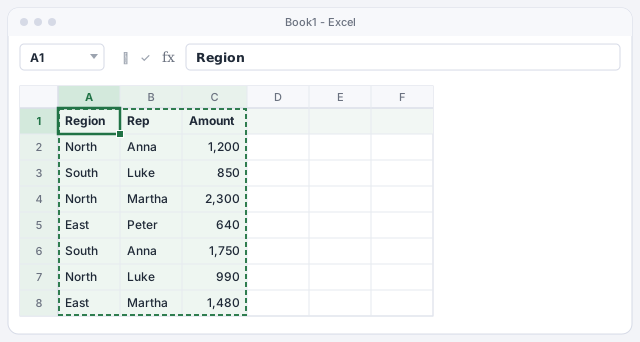
Older version? The ribbon filter (Data › Sort & Filter › Filter) and Remove Duplicates do something similar, but by hand and without updating themselves.
Filter one region's rows with FILTER
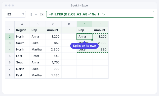
Type the headers Rep and Amount in E1 and F1. Then, in E2, type =FILTER(B2:C8,A2:A8="North") and press Enter.
The first argument is which columns you want to see (B2:C8); the second is the condition each row must meet (A2:A8="North"). Although you only typed in E2, the result fills E2:F4: Anna 1,200, Martha 2,300 and Luke 990. The spilled range is marked with a thin blue border.
Returns rep and amount for the rows whose region is North.
Type the region in a cell (for example H1) and use =FILTER(B2:C8,A2:A8=H1): change the cell and the report changes.
Add a message for when there are no results
If no row meets the condition, FILTER returns the #CALC! error. Avoid it with the third argument, which says what to show when the result is empty:
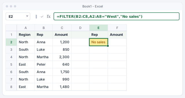
=FILTER(B2:C8,A2:A8="West","No sales")
Since there are no sales in the West region, E2 shows No sales. As soon as someone adds a West sale inside the range, it will appear in the list.
If there are no West rows, shows “No sales”.
Combine conditions with * (AND) and + (OR)
To require two conditions at once, wrap each one in parentheses and multiply them. North sales over 1,000:
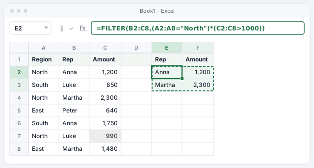
=FILTER(B2:C8,(A2:A8="North")*(C2:C8>1000))
The result is Anna 1,200 and Martha 2,300 (Luke is left out with 990). If you want either condition to count, add instead of multiplying: =FILTER(B2:C8,(A2:A8="North")+(A2:A8="South")) returns the North and South sales.
North region and amount greater than 1000.
North region or South region.
AND and OR don't work inside FILTER: they return a single TRUE or FALSE for the whole range. Use * and + with each condition in parentheses.
Sort the result with SORT
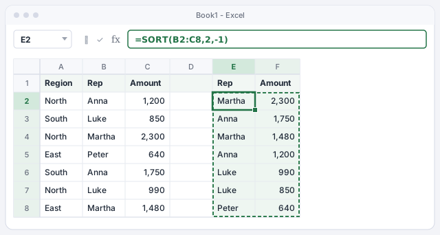
SORT takes a range, the column to sort by and the order (1 ascending, -1 descending). To see every sale from largest to smallest amount, type in E2: =SORT(B2:C8,2,-1). The 2 is the second column of the range (Amount), not column B of the sheet.
The real power is nesting: =SORT(FILTER(B2:C8,A2:A8="North"),2,-1) returns the North sales already sorted: Martha 2,300, Anna 1,200, Luke 990.
All sales, from largest to smallest amount.
North sales sorted from largest to smallest.
To sort by a column you won't display, use SORTBY: =SORTBY(B2:B8,C2:C8,-1) returns the reps sorted by amount.
Get a list without repeats with UNIQUE
UNIQUE returns each value once, in the order it first appears. Type =SORT(UNIQUE(A2:A8)) in E2 and you get the regions without repeats and in alphabetical order: East, North, South.
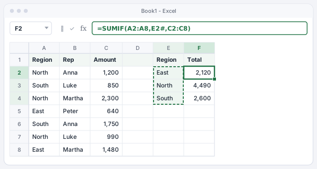
Now the trick: in F2 type =SUMIF(A2:A8,E2#,C2:C8). The # after E2 means “the whole range spilled from E2”. This formula spills too and gives you the total per region: 2,120, 4,490 and 2,600. If a new region shows up, it's added to both columns automatically.
Regions without repeats, in alphabetical order.
Total for each region in the list spilled from E2.
UNIQUE has a third argument: =UNIQUE(B2:B8,FALSE,TRUE) returns only the values that appear exactly once (in the example, Peter).
Fix the #SPILL! error
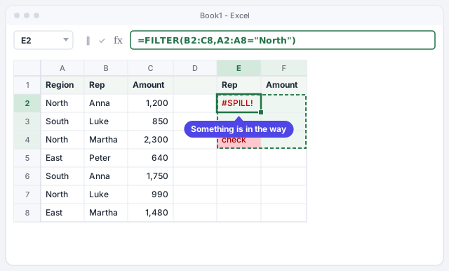
If any cell in the range where the result needs to spill isn't empty, the formula can't write over it and shows #SPILL!. Click the cell with the error: Excel draws a dashed border around the area it needs, and the warning icon offers Select Obstructing Cells.
Delete or move whatever is in the way (in the example, a forgotten note in E4) and the result appears instantly. Other causes: typing the formula inside an Excel table (spilled formulas don't work there) or the result running past the edge of the sheet.
Don't type inside a spilled range: any value you put there breaks the formula in the first cell.
Expert tips
- Use a table as the source. If you turn the data into a table named
Sales, type=FILTER(Sales,Sales[Region]="North")outside the table: every new row flows into the result automatically. See Excel tables. - Count what comes back.
=ROWS(E2#)tells you how many rows the spilled result has, and=COUNTA(UNIQUE(B2:B8))how many different reps there are (4 in the example). - Build dynamic reports with drop-down lists. Put a drop-down list of regions in a cell and use it as the
FILTERcondition: you get a report anyone can query without touching formulas. - Name the pieces. When a formula nests three functions,
LETlets you name each step so it reads better. We cover it in defined names and LET.
Common mistakes and how to fix them
The formula shows #NAME? as soon as you type it.
Your version of Excel doesn't have dynamic arrays (Excel 2019 or earlier) or the name is misspelled. Make sure you're using FILTER, SORT or UNIQUE in Microsoft 365, Excel 2021 or later.
FILTER returns #VALUE! when you combine conditions.
The condition ranges must have the same number of rows as the filtered range. If you filter B2:C8, the conditions must use A2:A8 and C2:C8, not A2:A10.
New rows you add below don't show up in the result.
The formula's range ends on row 8. Extend it or, better, turn the data into an Excel table and use references like Sales[Region], which grow on their own.
In Excel for Mac the functions are the same and are available in Microsoft 365 for Mac and Excel 2021 for Mac or later. You type the formulas exactly the same way.
Frequently asked questions
What's the difference between FILTER and the ribbon filter?
The filter in Data › Sort & Filter › Filter hides rows in the original data. FILTER leaves the data untouched and builds a filtered copy elsewhere that updates itself. For the classic filter, see sort and filter without scrambling your rows.
What happens if I open the file in an older Excel?
Results that were already calculated usually display, but the formulas can't be edited or recalculated normally. If the file will travel to older versions, copy the result and paste it as values.
Can I filter by text that contains a word?
Yes, by combining ISNUMBER and SEARCH: =FILTER(B2:C8,ISNUMBER(SEARCH("ar",B2:B8))) returns the rows whose rep contains “ar” (Martha, twice).
Can a dynamic array formula feed a chart or a drop-down list?
Yes. In a drop-down list's source you can type a spill reference such as =$E$2#, so the list always matches the current result. It's a neat way to keep drop-downs in sync with your data.
Official sources
Microsoft documentation consulted for this guide.
Saved only in this browser.