Drop-down lists and data validation: stop people typing what they shouldn't
Type the options in a column (ideally on another sheet), select the cells that will hold the list and go to Data › Data Tools › Data Validation. On the Settings tab choose Allow: List and, in Source, select the range of options (for example =Lists!$A$2:$A$5). Keep In-cell dropdown checked and click OK.
You share an orders sheet and, in the Status column, everyone types whatever they like: "Shipped", "shipped", "Shpd", "SHIPPED already". Then you try to filter or build a PivotTable and get four statuses that are really one. The problem isn't the people: it's that the sheet lets anyone type anything.
Data validation is like a doorman for each cell: it only lets in what meets your rules. Its most useful form is the drop-down list, an arrow that offers the allowed options so people pick one with a click.
In this guide you'll build a drop-down list that grows by itself, add a help message and an error alert, and learn to restrict amounts, dates and duplicates.
What you'll learn
- Create a drop-down list from a range on another sheet
- Add a custom help message and error alert
- Restrict amounts and dates, or block duplicates with a formula
- Find the data that was already wrong before you added the rule
Step by step
Type the options on a separate sheet
Create a sheet called Lists and type a header (Status) and, below it, one option per cell: Pending, Shipped, Delivered and Canceled. Keeping them apart stops anyone deleting them by accident and lets you reuse them.
Type them exactly as you want them to appear, in the order they'll show in the list.
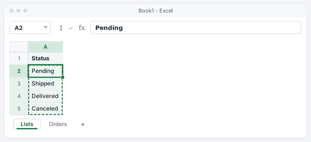
Turn the range into a table (Insert › Table). Then, when you add a new option below, every list based on it updates by itself.
Select the cells that will hold the list
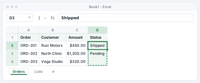
Go to the Orders sheet and select the status column, from D2 down to the last row you'll use (for example D2:D200). Leave out the header.
If you're working in an Excel Table, just select the column's cells: new rows will inherit the validation.
Open Data › Data Tools › Data Validation
On the Data tab, in the Data Tools group, click Data Validation. If you click the button's arrow, choose Data Validation... from the menu. The Data Validation dialog opens.

If the button is grayed out, the sheet is protected or a cell is still in edit mode. Press Esc or unprotect the sheet.
Choose Allow: List and select the source
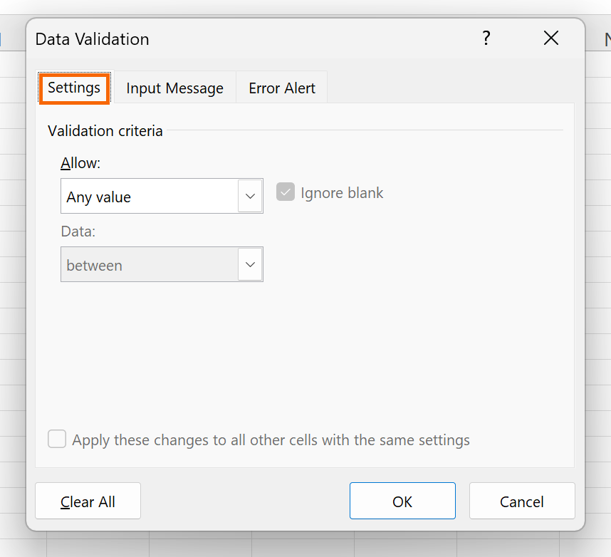
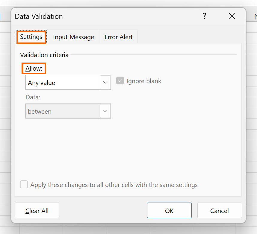
On the Settings tab, open Allow and choose List. Click in the Source box, go to the Lists sheet and select A2:A5 (no header). Excel fills in =Lists!$A$2:$A$5.
Keep Ignore blank (lets the cell stay empty) and In-cell dropdown (without it, no arrow appears) checked.
List source: the four options on the Lists sheet, as an absolute reference.
For short lists that won't change, you can type the options straight into Source, separated by commas: Yes,No.
Add a help message on the Input Message tab
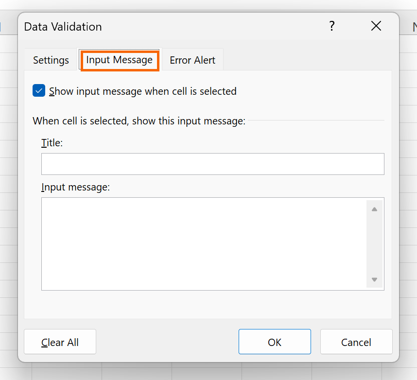
Switch to the Input Message tab. Keep Show input message when cell is selected checked and type a Title (Order status) and the Input message (Pick a status from the list). It shows up as a small yellow note when the cell is selected: instructions right where they're needed.
Decide what happens if someone types something else
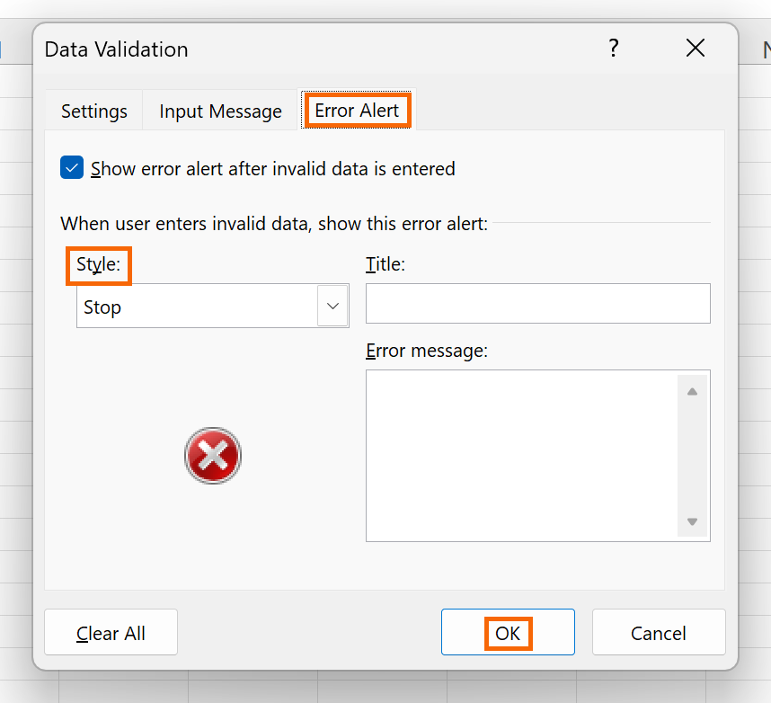
On the Error Alert tab, the Style sets how strict the rule is:
- Stop (red icon): won't accept a value outside the list.
- Warning: warns and asks whether to continue.
- Information: just informs and accepts the value.
Choose Stop, then write a title and a message that says what's allowed, not just that it's wrong. Click OK.
Test the list
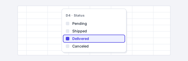
Click D4: the arrow appears to the right of the cell along with the help message. Choose Delivered. From the keyboard, Alt+↓ opens the list without touching the mouse.
Now type "delivered already" and press Enter: your error message appears and Excel rejects the value. Case doesn't matter: "delivered" is accepted.
Restrict amounts, dates and duplicates too
A list is only one of the Allow options. The others prevent plenty of typos:
- Decimal between
0and5000in the Amount column: no more 45000 instead of 450. - Date greater than or equal to
=TODAY(): blocks delivery dates in the past. - Text length: for example, a 5-character ZIP code.
- Custom: any formula that returns
TRUE. WithA2:A200selected,=COUNTIF($A$2:$A$200,A2)=1blocks a repeated order number.
Only accepts the order number if it isn't already in the column.
Find the data that was already wrong
Validation only checks what's typed from now on: whatever was already in the cells isn't reviewed. To see it, go to Data › Data Validation (the button's arrow) › Circle Invalid Data. Excel draws a red circle around every value that breaks the rule. Fix them and remove the circles with Clear Validation Circles.

Expert tips
- Lists that depend on another. If you pick Fruit in
B2and wantC2to offer only fruits, create a defined name Fruit for that range and use=INDIRECT(B2)as the source. More on names in defined names and LET. - A unique list that updates itself. In Microsoft 365, if you type
=SORT(UNIQUE(Orders!B2:B200))inLists!C2, you can use=Lists!$C$2#as the source: the#takes the whole result, however much it grows. - Copy only the validation. Copy a cell with the rule, select the destination and use Home › Paste › Paste Special... › Validation. Values and formatting stay untouched.
- Add colors. A conditional formatting rule that colors Canceled red and Delivered green turns the column into a traffic light.
- Lock it down. So nobody changes or removes the rule, protect the sheet and leave only the input cells unlocked.
Common mistakes and how to fix them
Someone pastes data over the cells and the validation disappears.
Pasting with Ctrl+V replaces the cell's rule too. Ask people to use Paste Special › Values, or reapply the validation and check with Circle Invalid Data.
The header shows up as one more option in the list.
The source includes row 1. Edit the rule and keep only the options, for example =Lists!$A$2:$A$5.
The drop-down arrow doesn't appear.
Check that In-cell dropdown is selected on the Settings tab.
You add a new option and it doesn't show up in the list.
You typed it outside the source range. Extend the range or, better, turn the options into a table so it grows on its own.
In Excel for Mac the path is Data › Data Validation, with the same three tabs (Settings, Input Message and Error Alert) and the same Allow options.
Frequently asked questions
How do I remove a drop-down list?
Select the cells, open Data › Data Validation and under Allow choose Any value. Click OK. Values already typed are kept.
Why does Excel let me type something that isn't in the list?
Either the error alert style is Warning or Information (both let you continue), or Show error alert after invalid data is entered is unchecked.
Can the list hold hundreds of options?
Yes, but scrolling a long list is slow. For long catalogs, sort the source alphabetically, or split it into two dependent lists (category, then item).
Can I sort the options alphabetically?
The list shows the options in the same order as the source. Sort the range on the Lists sheet (Data › Sort & Filter) and the list changes instantly.
Official sources
Microsoft documentation consulted for this guide.
Saved only in this browser.