A simple dashboard with a pivot table, a chart and a slicer
Turn the data into a table (Insert › Table), create a PivotTable on another sheet (Insert › PivotTable) and add a PivotChart from PivotTable Analyze › PivotChart. Insert a slicer for Region (PivotTable Analyze › Insert Slicer) and move the chart, the slicer and KPIs calculated with GETPIVOTDATA to a Dashboard sheet. Update everything with Data › Refresh All.
Every Monday someone asks “how are we doing this quarter?” and you open the sales sheet, filter, add up, paste a chart into an email… and on Tuesday they want the same thing for North only. A dashboard solves that: a single sheet with the key numbers, a chart and a few buttons to filter, which updates with one click when new data arrives.
Think of it as a car's dashboard: you don't see the engine, you see the speed and the fuel. The engine is your data and a PivotTable; the dashboard is the Dashboard sheet. In this guide you build a monthly sales dashboard from three pieces Excel already has: a PivotTable, a PivotChart and a slicer. No macros and no complicated formulas.
What you'll learn
- How to organize the workbook into three sheets: Data, Summary and Dashboard
- How to create the PivotTable and PivotChart that feed the dashboard
- How to calculate KPIs with GETPIVOTDATA that respect the filters
- How to connect one slicer to several PivotTables and refresh everything
Step by step
Turn the data into a table named Sales
Put the data on a sheet called Data: one row per sale, with Date, Region, Product and Amount. Click inside it and go to Insert › Tables › Table; check that My table has headers is ticked and click OK.
Then, in Table Design › Properties › Table Name, change Table1 to Sales. When you paste next month's sales underneath, it grows on its own and the PivotTable picks them up on refresh.
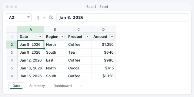
Dates must be real dates, not text. If they line up on the left, fix them before going on.
Create the PivotTable on a separate sheet
With a cell in the table selected, go to Insert › Tables › PivotTable. In the window, the Table/Range box already says Sales. Choose New Worksheet and click OK. Rename the new sheet Summary (double-click the tab).
This sheet is the “engine room”: nobody else needs to look at it. If you've never built a PivotTable, start with PivotTables in 5 minutes.
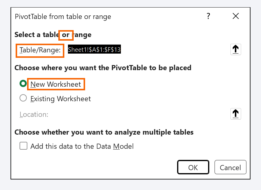
In older versions of Excel the window is called Create PivotTable; the options are the same.
Place the fields: months in rows, amount in values
In the PivotTable Fields pane on the right, drag Date to the Rows area. Excel groups the dates by month automatically (if it doesn't, right-click a date › Group… › Months). Drag Amount to Values: it shows up as Sum of Amount.
With first-quarter data you get: Jan $12,400, Feb $13,150, Mar $15,800 and a Grand Total of $41,350. Format the values as currency with right-click › Number Format….

Create the PivotChart and clean it up
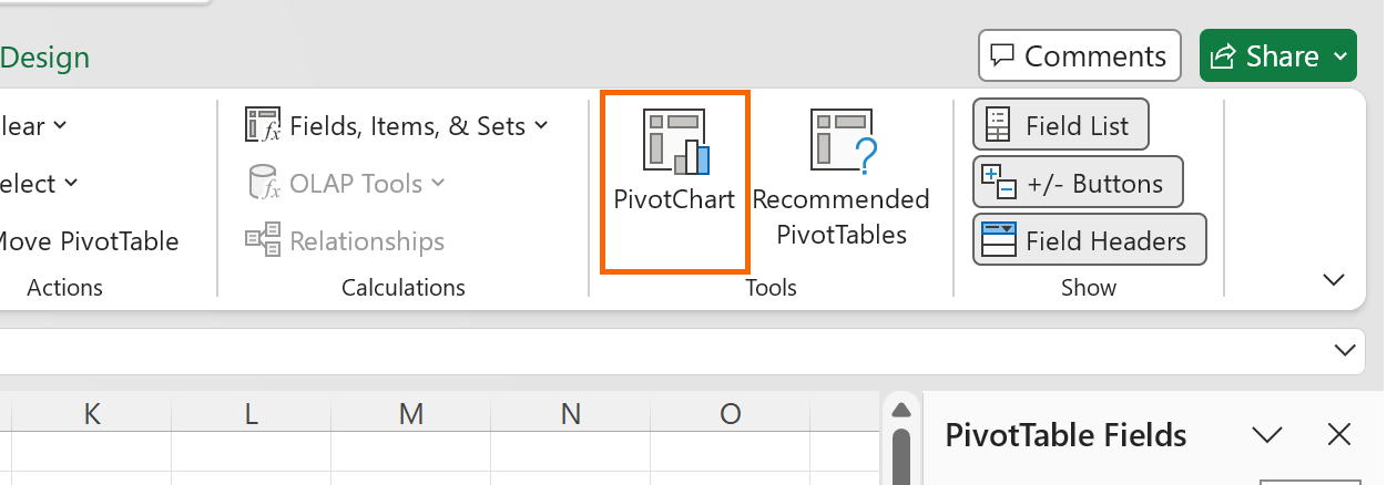
Click inside the PivotTable and go to PivotTable Analyze › Tools › PivotChart. Choose Clustered Column (or Line if the trend is what matters) and click OK. A PivotChart is a chart tied to the PivotTable: filter the table and the chart changes with it.
Remove the clutter: the legend (there's only one series) and the gray field buttons, from PivotChart Analyze › Show/Hide › Field Buttons. Give it a title that says what it shows, for example “Sales by month”.
Add a slicer for Region
A slicer is a panel of buttons that filters with one click. With the PivotTable selected, go to PivotTable Analyze › Filter › Insert Slicer, check Region and click OK.
Try it: click North and both the PivotTable and the chart show North only. Ctrl+click selects several regions; the crossed-out funnel icon at the top right of the slicer clears the filter.

Build the Dashboard sheet with KPIs that follow the filter
Create a sheet called Dashboard. Select the chart on Summary, cut it (Ctrl+X) and paste it (Ctrl+V) on Dashboard. Do the same with the slicer: they stay connected even on a different sheet.
Now the KPIs. In B2 type =, go to Summary and click the Grand Total: Excel builds a GETPIVOTDATA formula for you, which reads the value from the PivotTable even when it changes size. Type the target in B3 and the attainment in B4: 41,350 / 45,000 = 92%. Click North on the slicer and the sales KPI changes too.
Returns the grand total of the PivotTable that starts at A3 on the Summary sheet: $41,350.
Target attainment; format it as a percentage to see 92%.
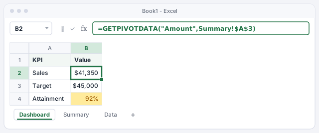
The target in B3 covers all regions. If you filter a single region, the attainment percentage is no longer comparable.
Connect the slicer to a second PivotTable
A dashboard usually has more than one view. Copy the PivotTable on Summary, paste it further down and swap Date for Product in Rows: now you have sales by product (and you can give it its own PivotChart).
To make the same slicer filter both, select it and go to Slicer › Report Connections. Check both PivotTables (PivotTable1 and PivotTable2) and click OK. One click on South and the whole dashboard tells South's story.
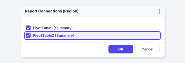
Give your PivotTables clear names in PivotTable Analyze › PivotTable (for example, PT_Months and PT_Products): in Report Connections you'll know which is which.
Polish the layout and update with Data › Refresh All
To make it look like a dashboard and not a spreadsheet, turn off View › Show › Gridlines, line up the chart, slicer and KPIs, and stick to a single highlight color.
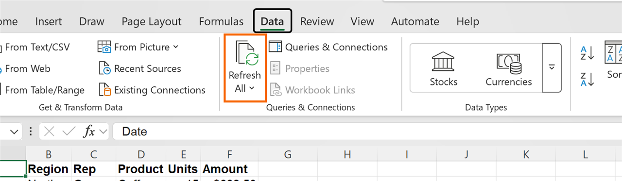
Most important: a PivotTable does not update by itself when the data changes. When you paste April's sales into the Sales table, go to Data › Queries & Connections › Refresh All. The PivotTables, the chart and the KPIs all update at once.
Expert tips
- Stop the columns from jumping. On refresh, the PivotTable resizes its columns and knocks the layout out of place. Right-click it › PivotTable Options… › Layout & Format tab › clear Autofit column widths on update.
- Refresh on open. In PivotTable Options › Data, check Refresh data when opening the file: anyone opening the dashboard always sees the latest data saved in the table.
- Filter by date too. PivotTable Analyze › Filter › Insert Timeline adds a bar for picking months or quarters by dragging. We cover it in slicers and timelines.
- AI for the first draft. Ask ChatGPT or Copilot which KPIs make sense for your business, but build the dashboard yourself on a PivotTable: that way you can check any number with a double-click, which opens the rows behind it.
Common mistakes and how to fix them
You add new sales and the dashboard still shows the old numbers.
PivotTables don't recalculate on their own. Go to Data › Queries & Connections › Refresh All. If they still don't show, check that you pasted them inside the Sales table and not below it.
The sales KPI shows #REF! after you change the PivotTable.
GETPIVOTDATA can't find the field or the PivotTable. Make sure Amount is still in Values and that the reference points to a cell inside the PivotTable (for example Summary!$A$3).
The slicer filters one chart but not the other.
The second PivotTable isn't connected. Select the slicer and check both in Slicer › Report Connections.
Clicking a PivotTable cell gives you a long formula instead of =Summary!B7.
That's GETPIVOTDATA, and it's what you want for a dashboard. If you prefer plain references, turn it off in PivotTable Analyze › PivotTable › Options › Generate GetPivotData.
In Excel for Mac you can create PivotTables, PivotCharts and slicers; the contextual tabs have the same names (PivotTable Analyze, Chart Design). Some options move around between versions: if you can't find a button, Control+click the object and use its shortcut menu.
Frequently asked questions
Why a PivotTable and not formulas like SUMIFS?
You can build dashboards with formulas, but a PivotTable gives you month grouping, PivotCharts and slicers for free, and it grows without you touching anything. For one-off KPIs, SUMIFS is a good complement.
Can I share the dashboard with my team?
Yes. Save the workbook to OneDrive or SharePoint and share it; slicers and charts also work in Excel for the web. If you don't want anyone touching the formulas, protect the Dashboard sheet and leave the slicers unlocked.
My GETPIVOTDATA formula returns #REF! when I copy it. Why?
The formula points to a specific sheet and cell. Check that your sheet is called Summary and that the PivotTable starts at A3; otherwise, delete the formula and build it again by typing = and clicking the Grand Total.
Does it work with data that arrives from another system every month?
Yes, and even better if you import it with Power Query: load the data into the table, click Refresh All and the query, the PivotTables and the dashboard all update in one go.
Saved only in this browser.