Slicers and timelines: button filters for your reports
Click inside the pivot table and go to PivotTable Analyze › Filter › Insert Slicer; tick the fields (for example, Region) and click OK. Each button filters the table with one click, and Ctrl+click selects several. For dates, use Insert Timeline in the same group and drag across the months you want to see.
You send a report with a pivot table and the next day someone asks for “the same, but North only”, and then “just February and March”. Pivot table filters work, but they're hidden behind a tiny arrow and nobody can see what's filtered. Whoever opens the file may read partial figures thinking they're totals.
A slicer is a panel of buttons that filters the pivot table with one click: one button per region, product or salesperson. A timeline does the same for dates: a bar of months (or quarters, or years) that you select by dragging. Both keep the current filter in plain sight, and a single one can control several pivot tables at once. They're the foundation of any dashboard.
What you'll learn
- Insert slicers to filter by region or product with one click
- Select several buttons and clear the filter
- Filter by month or quarter with a timeline
- Connect one slicer to several pivot tables and give it a tidy look
Step by step
Start with a pivot table that has something to filter
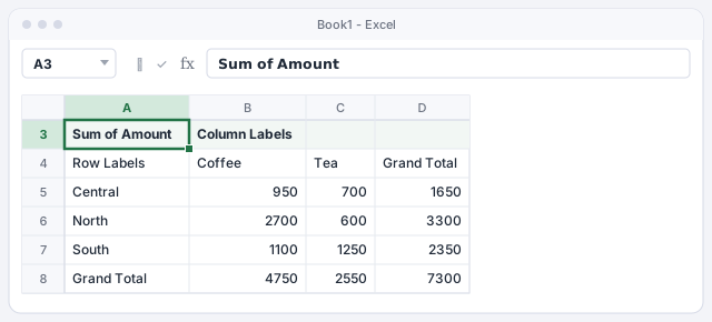
You need a pivot table built from an Excel table. If you don't have one yet, follow Pivot tables in 5 minutes. Here we use eight sample sales with Region in Rows, Product in Columns and Amount in Values: 7,300 in total.
Leave a few empty columns to the right of the pivot table: that's where the buttons will go.
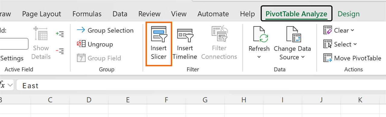
Insert a slicer
Click any cell in the pivot table so its contextual tabs appear. Go to PivotTable Analyze › Filter › Insert Slicer. You can also get there from Insert › Filters › Slicer.
Slicers also work on regular Excel tables, with no pivot table: with the cursor inside the table, use the same option on the Insert tab.
Tick the fields you want to filter by
The Insert Slicers dialog opens, with one field for each column in the source. Tick Region and Product and click OK. Excel creates one slicer per field, floating over the sheet; drag them by the edge into place.
Pick fields with few distinct values (regions, products, salespeople, statuses). A slicer with 300 customers is an endless list of buttons: the regular filter works better for that.

Filter with one click (or several)
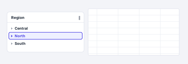
Click North: the pivot table shows only that region (Coffee 2,700, Tea 600, total 3,300) and the other buttons fade. To see several regions, hold Ctrl and click each one, or turn on the Multi-Select button in the slicer header.
To remove the filter, click Clear Filter (the funnel with an X, top right of the slicer). Slicers talk to each other: if a region sold no tea, clicking it would dim the Tea button in the other slicer.
Add a timeline for dates
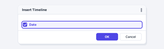
With the cursor in the pivot table, go to PivotTable Analyze › Filter › Insert Timeline. The Insert Timeline dialog lists only date fields: tick Date and click OK.
Timelines work only with pivot tables (not regular Excel tables) and need real dates. If Excel says there's no date field, check that your dates aren't stored as text.
Pick the time level and drag across the period
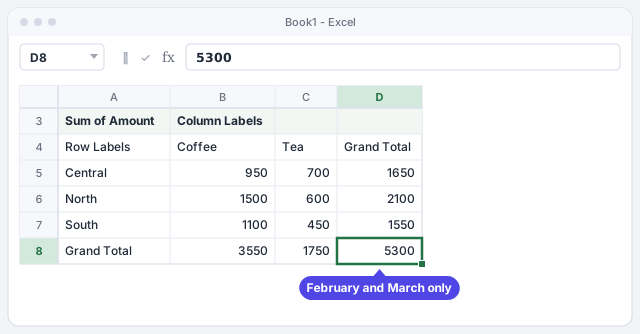
At the top right of the timeline there's a drop-down with the level: years, quarters, months or days. Choose MONTHS, click February and drag to March. The pivot table keeps just those two months: 5,300 in total (7,300 minus January's 2,000).
Timelines and slicers combine: if you also click North, you'll see only North in February and March (2,100). To see everything again, click Clear Filter on the timeline.
Connect one slicer to several pivot tables
If you have another pivot table built from the same source (for example, sales by salesperson), a single slicer can filter both. Click the slicer, go to the Slicer tab › Report Connections, tick the pivot tables it should control and click OK.
Timelines work the same way, from their own contextual tab. That's how you build a dashboard where one click on North changes every pivot table and PivotChart at once.

Arrange the buttons and give them a style
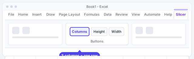
With the slicer selected, on the Slicer tab set Buttons › Columns to 3 so the three regions sit in one horizontal row, and adjust Height and Width. Pick a color from the styles gallery to tell each slicer apart.
Right-click › Slicer Settings… lets you change the header caption and hide items with no data. Place all slicers together, above or to the left of the report, so people read them before the numbers.
Expert tips
- Slicer and timeline on the same date. By default, Excel won't apply two filters to the same field. Turn it on in PivotTable Analyze › PivotTable › Options, Totals & Filters tab, Allow multiple filters per field checkbox.
- PivotCharts obey too. If you create a chart from the pivot table with PivotTable Analyze › PivotChart, the slicer filters it at the same time. Design ideas in charts people understand.
- Deleting a slicer doesn't delete data. Select it and press Delete; the pivot table and the source are untouched. Click Clear Filter first to make sure you're back to the full totals.
- Check what AI builds. If Copilot or ChatGPT helps you put a dashboard together, check in Report Connections that each slicer filters every table it should: it's the detail most often missed.
Common mistakes and how to fix them
Report Connections doesn't list the other pivot table.
Both pivot tables must come from the same source (the same Excel table). If you built the second one from another copy of the data, rebuild it from the original table.
Excel says there are no date fields when you insert a timeline.
Timelines need real dates. Convert dates stored as text in the source and refresh the pivot table.
Using the timeline clears the filter on the Date slicer (or vice versa).
Turn on Allow multiple filters per field in PivotTable Options, Totals & Filters tab.
Someone reads the filtered report thinking it shows totals.
Keep the slicers visible next to the table and click Clear Filter before sending the file if you want everything shown.
In Excel for Mac (Microsoft 365, 2021 and 2024) slicers and timelines are on the PivotTable Analyze tab. To select several buttons in a slicer, hold ⌘ instead of Ctrl.
Frequently asked questions
Can I use slicers without a pivot table?
Yes, on Excel tables: click inside the table and use Insert › Filters › Slicer. Timelines, on the other hand, only exist for pivot tables.
Do they work in Excel for the web?
You can use the slicers already in the file and create new slicers for regular pivot tables. To create them on Excel tables or Data Model pivot tables you need Excel for Windows or Mac.
What's the difference between a slicer and the Filters area?
They filter the same way, but a slicer shows what's selected at a glance and can control several pivot tables at once. The Filters area takes less space and suits fields with many values.
Official sources
Microsoft documentation consulted for this guide.
Saved only in this browser.