Clean data: remove duplicates and extra spaces, and split text into columns
To split, select the column and use Data › Data Tools › Text to Columns › Delimited, then pick the delimiter. To remove extra spaces, type =TRIM(B2) in a helper column and paste the result as values. To delete repeated rows, click in the data and use Data › Data Tools › Remove Duplicates. Do it in that order: extra spaces hide duplicates.
It happens every time you export a list from your billing system, your CRM or a web form: names with spaces in front, last and first name crammed into one cell, and customers listed twice. Then XLOOKUP finds nothing, the PivotTable overcounts and nobody knows why.
Cleaning data is like sorting groceries before putting them away: first you separate, then you trim what's left over, and finally you throw out the repeats. Excel has a tool for each. In this guide you clean a real customer list in three passes and learn why the order matters.
What you'll learn
- How to split “Last, First” into two columns with Text to Columns
- How to strip invisible spaces with the TRIM function without losing data
- How to see which rows are repeated before deleting them
- How to remove duplicates safely and decide which columns count
Step by step
Make a copy and see what needs cleaning
First, duplicate the sheet: right-click the tab › Move or Copy… › tick Create a copy. Cleaning data deletes and overwrites, and this way you always keep the original.
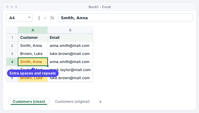
In the example, column A holds “Last, First” in one cell, there are extra spaces (row 4 has two after the comma and row 5 one at the end) and two customers appear twice.
Insert an empty column and open Text to Columns
Text to Columns writes its result into the columns to the right and overwrites whatever is there. Since the first name will go into column B, first right-click the B header › Insert: the email moves to C.
Now select A1:A6 and go to Data › Data Tools › Text to Columns. In the first step of the wizard choose Delimited (a character, here the comma, separates the pieces) and click Next.
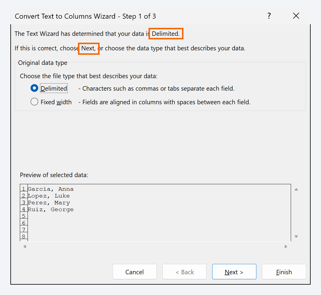
If you don't insert the empty column, Excel asks whether to replace the data at the destination. If you say yes, you lose the emails.
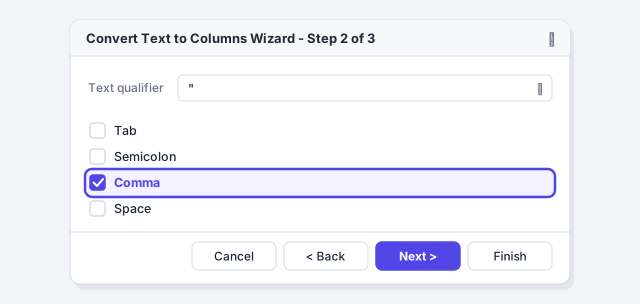
Choose the comma as the delimiter
Under Delimiters, tick Comma (you can untick Tab, which comes ticked). The preview below shows a line between last and first name. Click Next.
If your data uses a different character, such as a hyphen or a vertical bar, tick Other and type it in the box.
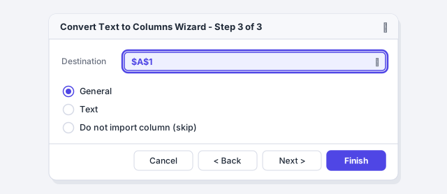
Check the format and destination, then click Finish
In the last step you can set the format of each column by clicking it in the preview. General works for almost everything. Make sure Destination is $A$1 and click Finish. Then rename the headers: A1 becomes Last name and B1 becomes First name.
If a column holds codes with leading zeros (ZIP codes like 02134, part numbers, IDs), set it to Text in this step or Excel will drop the zeros.
Strip extra spaces with TRIM
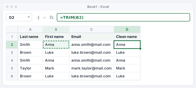
The first names now start with a space (the one that followed the comma) and some have more. They're invisible, but to Excel “ Anna” and “Anna” are different text. In helper column D type =TRIM(B2) and double-click the small square at the cell's corner to copy it down.
TRIM removes spaces at the start and end and leaves a single space between words. If the names also come in lowercase or all caps, use =PROPER(TRIM(B2)): “anna” becomes “Anna”.
Returns the name in B2 with no leading or trailing spaces.
Also capitalizes the first letter of each word.
Don't use TRIM on amount columns: the result is text and your totals will stop working.
Replace the names with the clean values
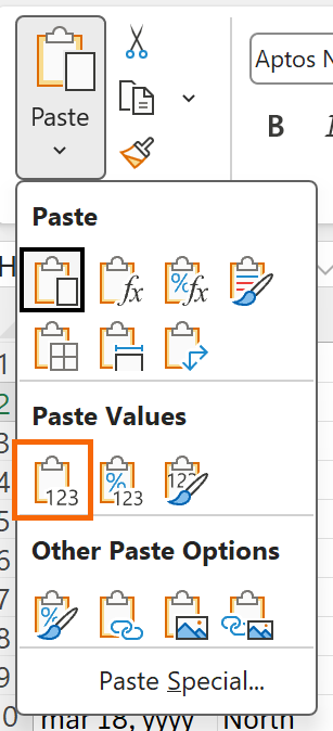
Column D is formulas: if you delete B, they'll show #REF!. To keep only the result, select D2:D6, copy it with Ctrl+C, click B2 and go to Home › Clipboard › Paste › Values. Column B now holds the clean names as plain text. Delete column D.
Check which rows are repeated with COUNTIF
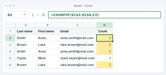
Before deleting, look at what you're about to delete. In D2 type =COUNTIF($C$2:$C$6,C2) and copy it down: it counts how many times that row's email appears in the whole column. Anything greater than 1 is a repeat.
To see them together, turn on the filter with Ctrl+Shift+L and sort by email. Once you've reviewed them, delete column D.
Counts how many times the email in C2 appears in the range C2:C6.
Delete the duplicates with Remove Duplicates
Click any cell in the data and go to Data › Data Tools › Remove Duplicates. Keep My data has headers ticked and choose which columns decide whether a row is a repeat: with all three ticked, only rows identical in everything are removed. Click OK.
Excel tells you how many duplicates it removed (here, 2) and how many unique values remain (3). It always keeps the first occurrence and deletes the ones below.
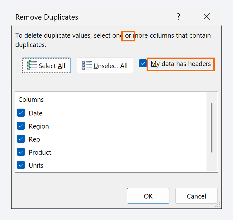
If two rows with the same email are the same customer to you even when the name is spelled differently, leave only the Email column ticked.
Expert tips
- Order matters: split, trim, dedupe.
Remove Duplicatescompares the exact text, spaces included. If you run it beforeTRIM, “Smith, Anna” and “Smith, Anna” both survive. It does not, however, care about upper or lower case. - In Microsoft 365, split with a formula.
=TEXTSPLIT(A2,", ")spreads the text across two cells using comma plus space as the delimiter, so no leading spaces are left. If the source changes, the result updates itself. - Some spaces TRIM won't remove. Data copied from web pages sometimes carries the non-breaking space. If it won't go away, combine it with
SUBSTITUTEandCHAR(160), or ask an AI for the exact formula and test it on three rows. More tricks in text functions. - To split by pattern, use Flash Fill. Type the first result by hand and use Data › Data Tools › Flash Fill (or Ctrl+E): how it works.
- Same cleanup every month? Do it once in Power Query and repeat it with one click: Power Query step by step.
Common mistakes and how to fix them
Text to Columns overwrote the column next to it.
Press Ctrl+Z right away. Insert as many empty columns to the right as pieces you'll get, and run the wizard again.
Remove Duplicates doesn't delete rows that look identical.
There are almost always extra spaces, at the start, at the end or doubled between words. Clean first with =TRIM(B2) and paste as values.
When you delete the original column, the clean column fills with #REF!.
They were still formulas. Undo with Ctrl+Z, copy the clean column, paste it with Paste › Values, and only then delete the original and the helper.
Amounts stop adding up after cleaning.
You applied TRIM to numbers and turned them into text. Use =VALUE(TRIM(D2)) or, if you see the green triangle, choose Convert to Number.
In Excel for Mac, Text to Columns and Remove Duplicates are on the same Data tab, and TRIM and COUNTIF work the same. Use ⌘+C to copy and the Paste menu on the Home tab to paste values.
Frequently asked questions
Does Remove Duplicates care about upper and lower case?
No. “anna” and “Anna” count as the same. Spaces do count, which is why you should use TRIM first.
Which row is kept when there are duplicates?
The first one, from top to bottom. If you want to keep the most recent, sort the data by date, newest first, beforehand.
My colleague's Excel shows formulas with semicolons. Why?
It depends on regional settings: in much of Europe and Latin America Excel uses ; between arguments and also translates function names. =COUNTIF($C$2:$C$6,C2) becomes CONTAR.SI with semicolons in Spanish Excel; the logic is identical.
Can I ask ChatGPT to clean the list for me?
For small lists with no personal data, yes. For customer data, check your company's policy first. The safest route is to ask it for the steps or the formula and apply them yourself in Excel, checking a few rows by hand.
Saved only in this browser.