Text functions: join, split and clean with CONCAT, TEXTJOIN, MID and TRIM
To join text use =A2&" "&B2 or =CONCAT(A2," ",B2); to join a whole list with a separator, =TEXTJOIN("; ",TRUE,C2:C5). To split, use =LEFT(A2,2), =MID(A2,4,4) and =RIGHT(A2,4), or combine them with SEARCH to cut at a character such as @. To clean up, =TRIM(A2) removes extra spaces and =PROPER(A2) fixes capitalization.
It happens every time someone sends you a list: first and last names arrive in separate columns and you need them together, or the other way round; product codes have the country and year stuck together; and names show up with extra spaces and in ALL CAPS. Fixing it by hand takes hours, and with a hundred rows it's out of the question.
Excel's text functions are like scissors and glue for cell contents: some join pieces, some cut at a position or at a character, and some clean. You write the formula once in the first row, drag it down, and Excel repeats the operation on every row.
In this guide you learn the six or seven functions that cover 90% of real cases, and how to turn the result into fixed text when you're done.
What you'll learn
- How to join text with &, CONCAT and TEXTJOIN
- How to extract a piece by position with LEFT, MID and RIGHT
- How to cut at a character (like the @ in an email) using SEARCH
- How to clean up spaces and capitalization with TRIM and PROPER
- How to turn formulas into fixed text before you share the file
Step by step
Join first and last name with the & operator
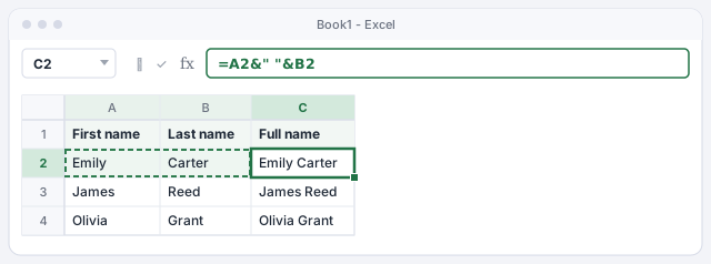
The & operator glues two pieces of text together. In C2 type =A2&" "&B2: it joins the first name in A2, a space (in quotes, because it's text) and the last name in B2. Press Enter and drag the fill handle (the small square at the bottom-right corner of the cell) down.
Without the " " in the middle you'd get “EmilyCarter”. It's the most common mistake.
First name, space and last name.
Use CONCAT to join several pieces at once
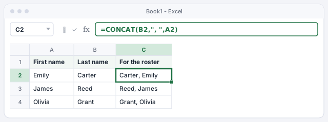
CONCAT does the same as &, but with the pieces separated by commas, which reads better when there are many. For the “Last, First” format of an official roster, type in C2: =CONCAT(B2,", ",A2).
CONCAT exists in Excel 2019 and later and in Microsoft 365. In older versions use CONCATENATE, which works the same: =CONCATENATE(B2,", ",A2).
Returns Carter, Emily.
Combine a whole list into one cell with TEXTJOIN
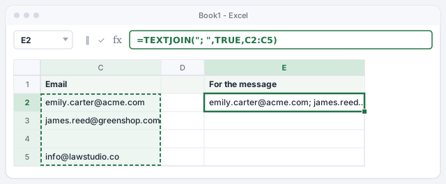
When you want to paste every email address in a column into the “To” field of a message, use TEXTJOIN. Its arguments are: the delimiter, whether to skip empty cells, and the range. In E2 type =TEXTJOIN("; ",TRUE,C2:C5).
With TRUE, the empty cell C4 is skipped and you don't get a “; ;” in the middle. Copy the result and paste it into Outlook: done. TEXTJOIN is available in Excel 2019, 2021, 2024 and Microsoft 365.
Joins the emails with semicolons, skipping empty cells.
Extract pieces by position with LEFT, MID and RIGHT
If every code has the same shape, like US-2026-0457 (country, year and number), cut by position:
=LEFT(A2,2)returns the first 2 characters:US.=MID(A2,4,4)returns 4 characters starting at the 4th:2026. The order is text, start position and number of characters.=RIGHT(A2,4)returns the last 4:0457.
Count positions including the hyphens: U is 1, S is 2, the hyphen is 3.
Country code.
Year: 4 characters from position 4.
Order number.

These functions always return text, which is why 0457 keeps its zero. If you need a number to calculate with, wrap the formula in VALUE: =VALUE(RIGHT(A2,4)).
Cut at a character with SEARCH (email user and domain)
When the pieces don't have a fixed length, find the character that separates them. SEARCH("@",B2) returns the position of the @. With that:
- User:
=LEFT(B2,SEARCH("@",B2)-1), everything before the @. - Domain:
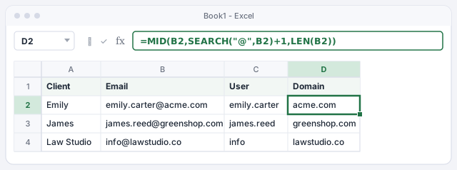
=MID(B2,SEARCH("@",B2)+1,LEN(B2)), everything after it.LENgives the total length; asking for too many characters doesn't cause an error.
In Microsoft 365 and Excel 2024 it's easier: =TEXTBEFORE(B2,"@") and =TEXTAFTER(B2,"@"). The SEARCH version works in any Excel.
Everything before the @.
Everything after the @.
If a cell doesn't contain the character, SEARCH returns #VALUE!. Wrap the formula in IFERROR to show a message instead.
Clean up spaces and capitalization with TRIM and PROPER
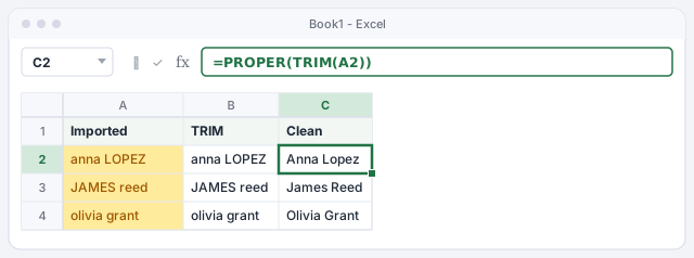
Data copied from another system often brings spaces at the start, at the end or doubled between words. They're invisible, but they stop XLOOKUP from finding anything. =TRIM(A2) removes them and leaves a single space between words.
For capitalization, PROPER capitalizes the first letter of each word, UPPER turns everything into capitals and LOWER into lowercase. You can nest them, that is, put one inside another: =PROPER(TRIM(A2)) cleans and fixes in one go.
Removes extra spaces.
Cleans up and capitalizes each word.
To remove non-printing characters (odd line breaks from legacy systems), add CLEAN: =TRIM(CLEAN(A2)).
Turn formulas into fixed text with Paste Values
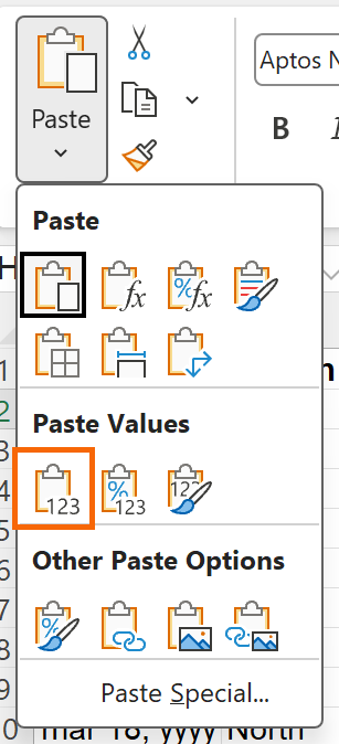
Once the result looks right, it's worth keeping it as plain text: that way you can delete the original columns without everything turning into #REF!. Select the column with the formulas, copy it with Ctrl+C and, without moving, go to Home › Clipboard › Paste (the arrow below it) › Paste Values › Values.
The formulas disappear and only the text remains. Now you can delete the source columns.
Do this last. Once pasted as values, the results no longer update if the original data changes.
Expert tips
- Try Flash Fill first. Type the result for the first row by hand and use Data › Data Tools › Flash Fill (or Ctrl+E): Excel guesses the pattern. It's ideal for a one-off fix; formulas are better when the data keeps changing. More in Flash Fill.
- Join numbers with their format.
="Total: "&TEXT(D2,"$#,##0.00")shows “Total: $1,250.00”. WithoutTEXT, Excel would paste “1250”. - Substitute instead of cutting.
=SUBSTITUTE(A2,"-","")removes every hyphen from a code, phone number or ID in one go. - Ask AI for the formula with an example. Tell ChatGPT “A2 contains US-2026-0457 and I want 2026”. Then check three rows by hand. More in asking AI for formulas.
Common mistakes and how to fix them
When you join first and last name they come out stuck together, like EmilyCarter.
The space in quotes is missing: =A2&" "&B2. Same with CONCAT: =CONCAT(A2," ",B2).
TRIM doesn't remove a space you can clearly see.
It's usually a non-breaking space (character 160) copied from a web page. Open Replace with Ctrl+H, in Find what type Alt+0160 on the numeric keypad, leave Replace with empty and click Replace All.
You delete the original column and the formulas show #REF!.
Before deleting, turn the result into text with Home › Paste › Paste Values › Values. If you already deleted it, undo with Ctrl+Z.
The year extracted with MID won't add up.
Text functions return text. Convert it to a number with =VALUE(MID(A2,4,4)).
In Excel for Mac the functions have the same names and work the same way. The copy shortcut becomes ⌘+C, and Replace is under Edit › Find › Replace.
Frequently asked questions
What's the difference between CONCAT, CONCATENATE and &?
None in the result. CONCAT is the modern version (Excel 2019 and later) and also accepts whole ranges; CONCATENATE still works for compatibility; & is the shortest for two or three pieces.
What's the difference between SEARCH and FIND?
Both return the position of one piece of text inside another. SEARCH isn't case-sensitive and FIND is. To look for an @ or a hyphen, either one works.
Can I split text into several columns without formulas?
Yes: Data › Data Tools › Text to Columns cuts it at a delimiter in one go. The result is fixed, whereas formulas update if the data changes. We cover it in cleaning data.
A formula I copied uses semicolons and Excel rejects it. Why?
Formulas from Spanish or European sources use ; as the separator. In US and UK Excel, replace them with commas, as in =CONCAT(B2,", ",A2).
Official sources
Microsoft documentation consulted for this guide.
Saved only in this browser.