Freeze Panes: keep the header row visible when you scroll down
To lock only row 1, go to View › Freeze Panes › Freeze Top Row. To lock rows and columns at once, select the cell just below and to the right of what you want to keep (for example, C2 for row 1 and columns A and B) and choose View › Freeze Panes › Freeze Panes. To remove it, choose View › Freeze Panes › Unfreeze Panes.
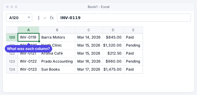
It happens as soon as a list runs past one screen: you scroll down to row 120 and can no longer tell whether that column was the invoice date or the due date, or whether the amount includes tax. You scroll up, check the header, scroll back down… and lose your place.
Freeze Panes is like putting a clipboard clip at the top of the sheet: the header row (and, if you like, the first columns) stays put while everything else scrolls underneath. It doesn't change your data or how it prints; only how you see it on screen.
In this guide you'll lock the header row in two clicks, learn the rule for freezing rows and columns at the same time, and find out how to undo it.
What you'll learn
- How to lock the header row with Freeze Top Row
- How to lock the first column, or several rows and columns at once
- The selected-cell rule: what stays put and what scrolls
- How to remove it with Unfreeze Panes
Step by step
Spot the problem: you scroll and the headers vanish
In the example you have an invoice log with hundreds of rows: Invoice, Customer, Date, Amount and Status. As soon as you scroll to row 120, row 1 with the headers leaves the screen and you only see loose numbers and names.
Before freezing, go back to the top of the sheet with Ctrl+Home, so row 1 is the first visible row.
Open View › Freeze Panes
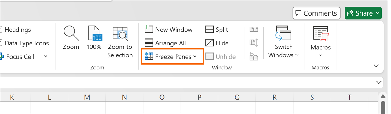
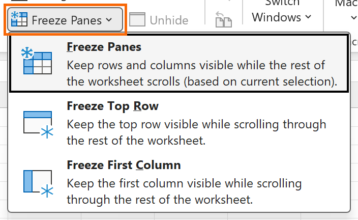
Go to the View tab. In the Window group you'll see the Freeze Panes button with an arrow. Click it to open its three options.
If the button is grayed out, you're probably in Page Layout view. Switch to View › Workbook Views › Normal.
Choose “Freeze Top Row” to lock the headers
Choose Freeze Top Row. A thin line appears under row 1. Now scroll down with the mouse wheel: the header row stays at the top and the data scrolls underneath.
If what you need is to always see column A (for example, the invoice number) while scrolling to the right, choose Freeze First Column.
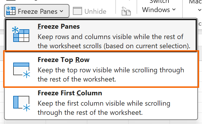
Freeze Top Row locks whichever row is at the top of the screen at that moment, not necessarily row 1. If you were at row 50, you'll lock row 50.
To lock rows and columns at once, select the key cell
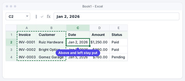
The two previous options don't combine: choosing one replaces the other. To lock the header row and the Invoice and Customer columns, use this rule: Excel freezes everything above and to the left of the selected cell.
- Click
C2(below row 1 and to the right of columnsAandB). - Go to View › Freeze Panes › Freeze Panes.
Other examples: A3 locks rows 1 and 2; B2 locks row 1 and column A.
Check that it works in both directions
Scroll down with the mouse wheel: the header row stays at the top. Scroll right (wheel with Shift held down, or the horizontal scroll bar): the Invoice and Customer columns stay on the left. You'll see a horizontal line under row 1 and a vertical one after column B: those are the edges of the frozen area.

Frozen panes are saved with the file: whoever opens it next will see the headers locked just like you do.
Remove it with “Unfreeze Panes”
When you no longer need it, or want to change what's locked, go to View › Freeze Panes › Unfreeze Panes. While something is frozen, the first option in the menu changes to that name.
To lock a different area, unfreeze first and then freeze again with the new cell selected.
Expert tips
- With tables, you barely need it. If your data is an Excel table and a table cell is selected, the column letters are replaced by your headers as you scroll. Still, freezing row 1 keeps the headers visible even when the cursor is outside the table.
- To compare distant areas, use Split. View › Window › Split divides the sheet into areas that scroll independently: you can see row 5 and row 900 at the same time. Click Split again to remove it.
- Paper is a different setting. Freezing only affects the screen. To repeat the headers on every printed page, use Page Layout › Print Titles: see print without cut-offs.
- Keyboard route. Press Alt, then W, F to open the Freeze Panes menu, and then R for Freeze Top Row or C for Freeze First Column.
Common mistakes and how to fix them
Row 37 got locked instead of the header row.
You used Freeze Top Row while the sheet was scrolled down. Choose Unfreeze Panes, press Ctrl+Home to go back to the top and freeze again.
You lock the top row, then the first column, and the row is no longer locked.
The two options replace each other. To lock both, select B2 and use Freeze Panes › Freeze Panes.
Half the screen got frozen and there's hardly any room left to scroll.
The selected cell was too far down or to the right. Unfreeze, select the cell just below the headers (for example, A2 or B2) and freeze again.
In Excel for Mac the same options (Freeze Panes, Freeze Top Row and Freeze First Column) are on the View tab, and the selected-cell rule is identical.
Frequently asked questions
Can I freeze a row other than the first one, such as row 4?
Yes, as long as you lock everything from the top down to it. Select A5 and choose Freeze Panes › Freeze Panes: rows 1 to 4 stay locked. You can't lock a single row in the middle on its own.
Does Freeze Panes affect printing?
No. It only changes what you see on screen. To repeat the headers on every printed page, use Page Layout › Print Titles.
Does it apply to every sheet in the workbook?
No. Each sheet has its own setting. If you want locked headers on several sheets, repeat the steps on each one.
Why is the Freeze Panes button grayed out?
Usually because you're in Page Layout view or still editing a cell. Press Esc to leave the cell and switch to View › Normal.
Saved only in this browser.