Subtotals and grouping rows: reports that collapse and expand
Sort the list by the grouping column (for example, Region) and go to Data › Outline › Subtotal. Set “At each change in” to Region, “Use function” to Sum and check the Amount column. Excel inserts a total row per group using SUBTOTAL plus a grand total, and adds the 1, 2 and 3 buttons on the left to collapse and expand the detail.
You have a sales list with hundreds of rows and someone asks for “the total by region, but with the detail available”. The usual approach is inserting rows by hand, typing sums one by one and hoping nobody adds a sale in the middle. The next day, the totals no longer add up.
Excel has a tool built for exactly this: Subtotal. It works like the collapsible table of contents of a book: you see the chapters (the group totals) and, if you want, open one to read the pages (the detail rows). In this guide you add subtotals in one click, learn to collapse the report by level, copy only the totals and group rows or columns by hand.
What you'll learn
- How to insert subtotals by group with Data › Outline › Subtotal
- Why the SUBTOTAL function never counts totals twice
- How to collapse and expand the report with the level buttons
- How to copy only the total rows and group rows or columns by hand
Step by step
Sort the list by the column that defines the groups
Subtotal creates a total every time the value changes in a column. If the list isn't sorted, you'll get a “North Total” every few rows. Click any cell in the Region column and go to Data › Sort & Filter › Sort…. Sort by Region, A to Z, and click OK.
In the example, the two North sales and the three South sales end up together.
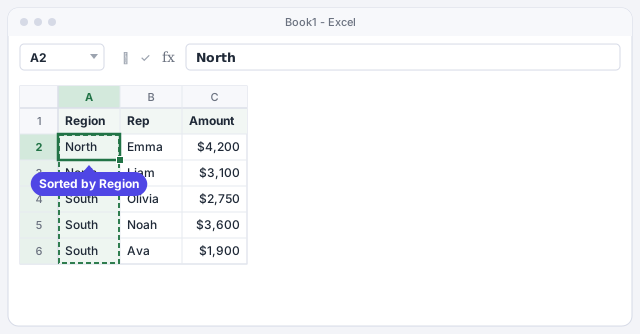
Subtotal doesn't work inside an Excel table (the button is grayed out). If your data is a table, convert it first with Table Design › Tools › Convert to Range.
Open Data › Outline › Subtotal
With any cell in the list selected, go to the Data tab and, in the Outline group (on the right of the ribbon), click Subtotal. Excel selects the whole data block for you and opens the Subtotal window.
An outline is the structure of levels that lets you collapse and expand rows; Subtotal builds it for you.

Pick the group, the function and the column to total
Fill in the three fields at the top:
- At each change in: Region (the column you sorted by).
- Use function: Sum. You can also choose Count, Average, Max or Min.
- Add subtotal to: check Amount and clear the rest.
Leave Replace current subtotals and Summary below data checked. If you'll print one region per page, also check Page break between groups. Click OK.

Check the totals: Excel uses the SUBTOTAL function
Excel inserts a North Total row and a South Total row under each group, plus a Grand Total at the end. Click C4 and look at the formula bar: it doesn't say SUM, but =SUBTOTAL(9,C2:C3). The 9 means “sum”.
The clever part is the grand total: =SUBTOTAL(9,C2:C8) also covers the total rows, but SUBTOTAL ignores other subtotals, so nothing is counted twice. Check it: 7,300 + 8,250 = $15,550.
Adds the North sales: 4,200 + 3,100 = $7,300.
Adds the South sales: 2,750 + 3,600 + 1,900 = $8,250.
Grand total: skips the subtotal rows and returns $15,550.
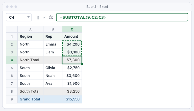
Collapse and expand with the 1, 2 and 3 buttons
To the left of the row numbers you now have buttons labeled 1, 2 and 3, plus − signs next to each group:
- 1: only the grand total.
- 2: the totals by region (what your boss wants to see).
- 3: all the detail.
The + and − signs open or close a single group. You can also use Data › Outline › Show Detail and Hide Detail with a cell in the group selected.

If you don't see the level buttons, go to File › Options › Advanced and, under the display options for this worksheet, turn on “Show outline symbols if an outline is applied”.
Copy only the totals with Go To Special
Click button 2 to see only the totals. If you copy and paste now, Excel also pastes the hidden rows. To avoid that, select the visible block and go to Home › Editing › Find & Select › Go To Special…. Choose Visible cells only and click OK.
Now copy (Ctrl+C) and paste (Ctrl+V) into another sheet or an email: only North Total, South Total and Grand Total come through.

Group rows or columns by hand with Data › Outline › Group
You don't always want automatic totals. If your sheet already has its own sums (for example, a budget with columns from January to December and one column per quarter), you can build the collapsing yourself. Select the January to March columns and go to Data › Outline › Group. If you selected loose cells instead of whole columns, Excel asks whether to group Rows or Columns.
A bar with a − sign appears above the columns: one click and the quarter collapses down to its total.
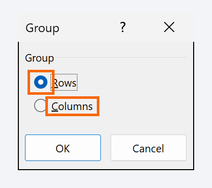
Shortcut to group the selection: Alt+Shift+Right Arrow. To ungroup: Alt+Shift+Left Arrow.
Remove the subtotals or the outline when you're done
To get back to the original list, select a cell in the data, open Data › Outline › Subtotal again and click Remove All. Excel deletes the total rows and the outline, and leaves your data untouched.
To remove a manual grouping, use Data › Outline › Ungroup with the rows or columns selected, or Ungroup › Clear Outline to remove every level on the sheet.

Expert tips
- Two levels of subtotals. Sort by Region and then by Rep. Apply Subtotal by Region; then open it again, choose Rep and clear Replace current subtotals. You get totals per rep inside each region and one more level button.
- Use SUBTOTAL outside this tool too. Under a filtered list,
=SUBTOTAL(9,C2:C100)adds only the rows still visible after filtering, whichSUMdoesn't do. With109instead of9it also ignores rows you hide by hand. - Auto Outline. If your sheet already has total formulas in sensible places, Data › Outline › Group › Auto Outline builds the levels for you without inserting rows.
- Need regions by month? Subtotal falls short there: use a PivotTable, which summarizes in two dimensions and doesn't touch your data.
Common mistakes and how to fix them
A “North Total” appears every few rows, over and over.
The list wasn't sorted by the grouping column. Click Subtotal › Remove All, sort by Region and apply Subtotal again.
The Subtotal button is grayed out.
Your data is an Excel table. Go to Table Design › Tools › Convert to Range and try again.
When you paste the totals into another sheet, all the detail rows come along.
Before copying, use Home › Editing › Find & Select › Go To Special › Visible cells only.
The grand total is double what it should be.
Someone replaced SUBTOTAL with SUM in the last row. Put back =SUBTOTAL(9,C2:C8) or apply Subtotal again.
In Excel for Mac the path is the same: Data › Subtotal (or Data › Outline › Subtotal, depending on window width) and Data › Group. The 1, 2 and 3 level buttons and the + and − signs work the same way. The Windows Alt shortcuts don't carry over directly: use the ribbon buttons.
Frequently asked questions
What's the difference between Subtotal and a PivotTable?
Subtotal inserts total rows inside your own list and lets you collapse it. A PivotTable builds a separate summary without touching the data, and can cross two dimensions (region by month). For a quick, printable report, Subtotal; for analysis, a PivotTable.
What do 9 and 109 mean in SUBTOTAL?
The first argument picks the operation: 9 is sum, 1 average, 2 count numbers, 4 max, 5 min. Adding 100 (109, 101…) also ignores rows hidden by hand. Rows hidden by a filter are always ignored.
Will the totals update if I change an amount?
Yes. The total rows are ordinary SUBTOTAL formulas, so they recalculate instantly. If you add a whole new row, insert it inside its group so it falls within the formula's range.
Can I put the total above each group instead of below?
Yes. In the Subtotal window, clear Summary below data before clicking OK.
Saved only in this browser.