A self-grading multiple-choice quiz in Excel (drop-down lists and automatic score)
Type the questions in one column, add a drop-down list in the next one with Data › Data Validation › Allow: List and Source a,b,c,d, and put the answer key in another column. Score each row with =IF(C2=E2,1,0), add up the correct answers and calculate the grade with ROUND. Finally, hide the key and protect the sheet with Review › Protect Sheet.
Grading 30 quizzes by hand means counting right answers, doing the math and counting again because something doesn't add up. If the quiz already lives in Excel, the sheet can do that work for you: the student or coworker picks their answers and the score appears on its own.
The idea is simple, like the see-through answer template some teachers lay over an answer sheet: one column with the student's answers, a hidden one with the right answers, and a formula that compares them row by row. You only need three tools you may already know: a drop-down list, the IF function and sheet protection.
In this guide you'll build a 10-question quiz scored out of 10, with right and wrong colors that switch on at the end and a hidden answer key. It works the same for a class, an internal training session or certification prep.
What you'll learn
- Set up the quiz sheet with a, b, c and d answers in a drop-down list
- Score each question with IF and total the correct answers with SUM or SUMPRODUCT
- Calculate a grade out of 10, rounded with ROUND
- Color right and wrong answers only when you choose
- Hide the key, protect the sheet and hand out the quiz
Step by step
Set up the sheet: question, answer, point and key
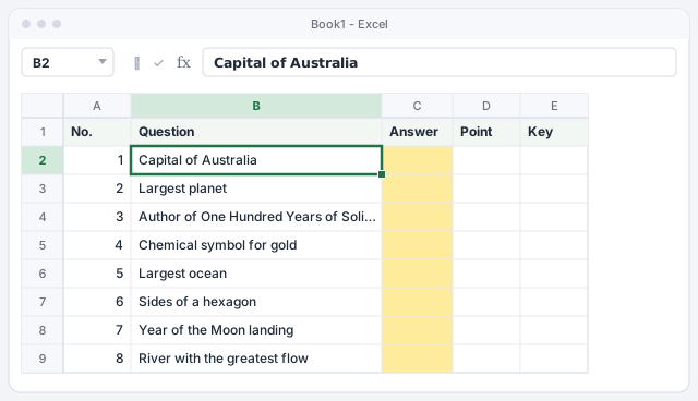
Create five columns: No. (A), Question (B), Answer (C), Point (D) and Key (E). Type the 10 questions in B2:B11. If you want the options visible in the cell itself, type them under the question with Alt+Enter (a line break inside the cell): a) Sydney b) Canberra c) Melbourne d) Perth.
Leave column C blank with a soft fill: it's the only place the quiz taker will type.
If you ask ChatGPT or Copilot for the questions, ask for the answer key as a separate list too, and check it yourself: AI sometimes marks a wrong option as correct.
Add an a, b, c, d drop-down list to the answers
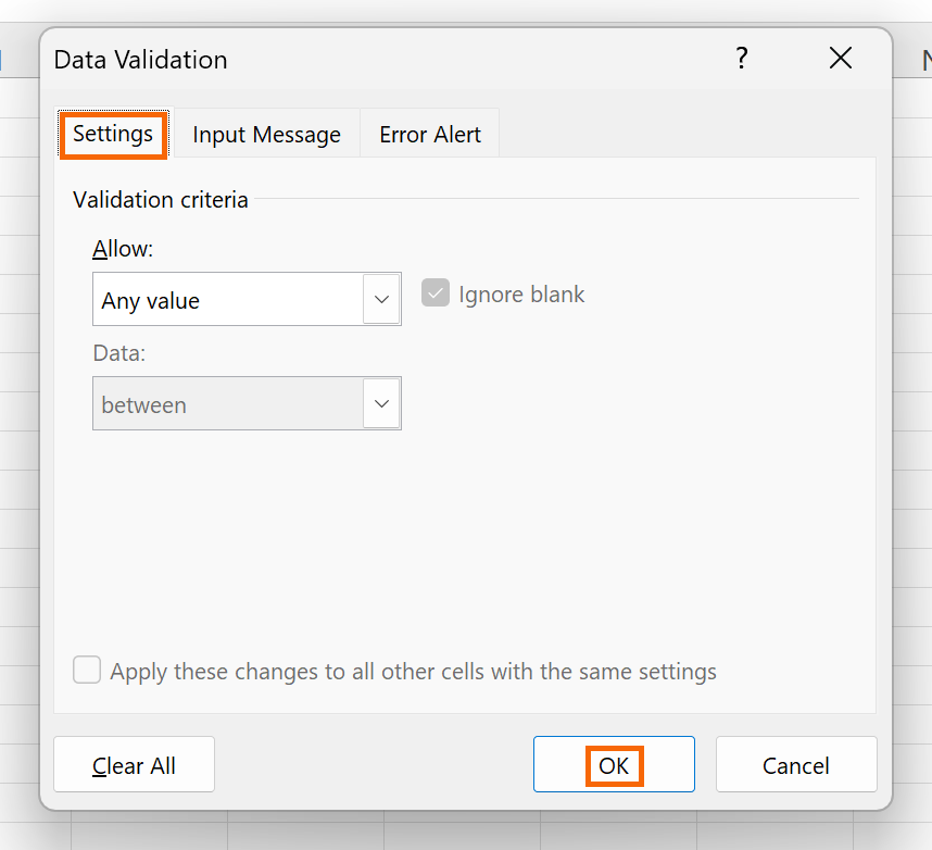
Select C2:C11 and go to Data › Data Tools › Data Validation. On the Settings tab, choose Allow: List and type a,b,c,d in Source. Keep In-cell dropdown checked.
On the Error Alert tab, keep the Stop style and type “Pick a, b, c or d”. That way nobody can answer “B I think” or “Canberra”, which the formula couldn't grade. For every validation option, see the guide to drop-down lists and data validation.
Case doesn't matter: if someone types B, Excel accepts it and the grading counts it the same as b.
Type the answer key in column E
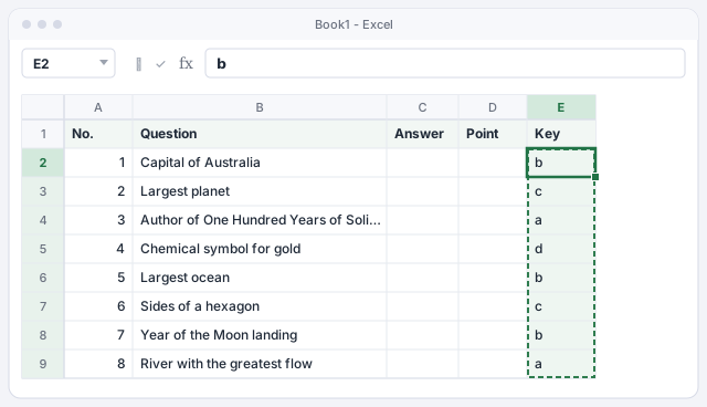
In E2:E11 type the correct letter for each question, lowercase and with no spaces: in this example, b, c, a, d, b, c, b, a, d, a. This column is your grading template: you'll hide it before handing out the quiz.
Check the key twice. A mistake here costs everyone an unfair point, and on a sheet that grades itself nobody notices until someone complains.
A trailing space after the letter (“b ”) means the answer never matches. If one question scores 0 for everybody, check that key cell.
Score each question with IF
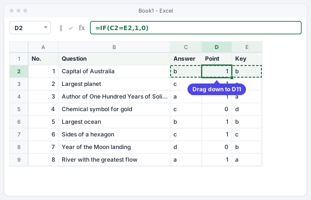
In D2 type =IF(C2=E2,1,0): if the answer matches the key, it's worth 1; otherwise, 0. An unanswered question also scores 0, because an empty cell doesn't match any letter. Drag the fill handle down to D11.
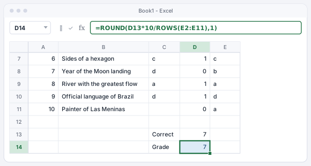
In the example, the quiz taker missed question 4 (picked c, it was d) and question 7 (picked d, it was b). If IF is new to you, see the IF function step by step.
1 point if the answer matches the key; 0 if it doesn't or is blank.
Total the correct answers and calculate the grade out of 10
In D13 add up the points with =SUM(D2:D11). If you'd rather skip the point column, a single formula does the same job: =SUMPRODUCT(--(C2:C11=E2:E11)). The comparison returns a list of TRUE and FALSE; the double minus (--) turns them into 1 and 0, and SUMPRODUCT adds them up. Another option is =COUNTIF(D2:D11,1).
In D14 calculate the grade with =ROUND(D13*10/ROWS(E2:E11),1). ROWS counts the questions, so the formula still works with 12 or 25 of them: 8 right out of 12 would give 6.7. In the example, 7 right out of 10 gives a 7.
Counts the correct answers without needing the point column.
Grade out of 10 with one decimal, for any number of questions.
Color right and wrong answers when you want to reveal them
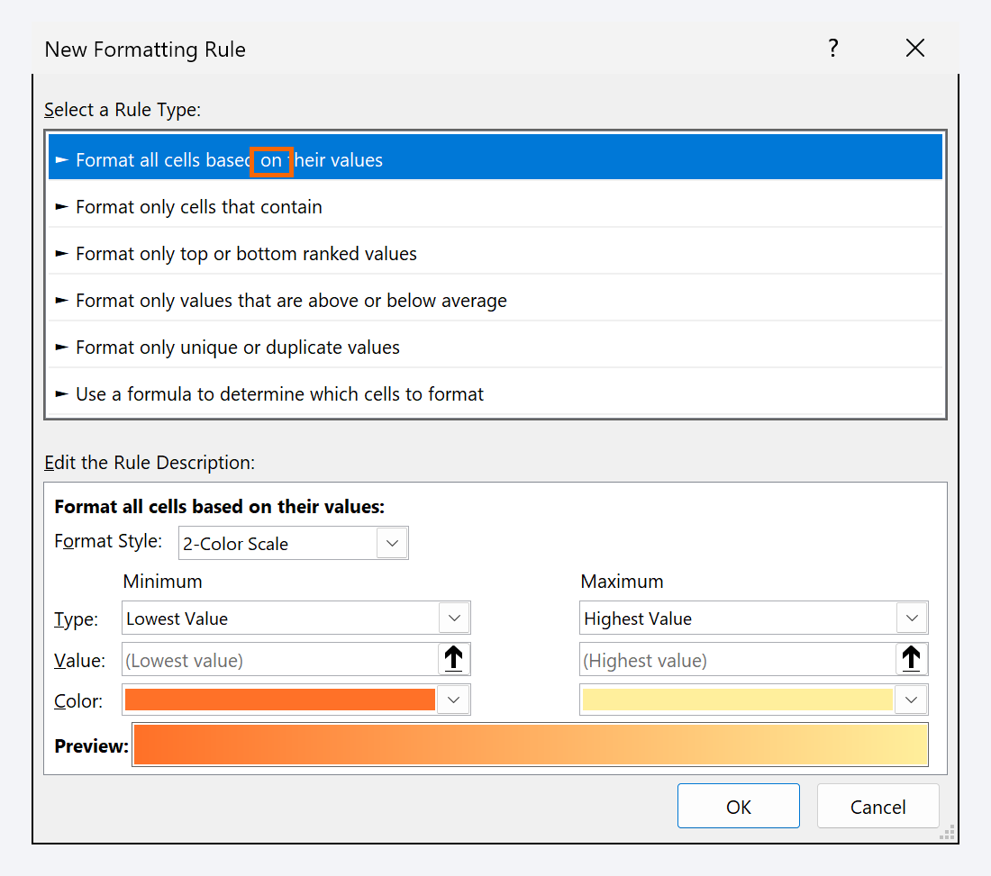
Type Grade it in G1 and give H1 a drop-down list with Yes,No (start it at No). Select C2:C11 and go to Home › Conditional Formatting › New Rule.... Choose Use a formula to determine which cells to format, type the green formula, click Format... and pick a green fill. Repeat with a second rule for red.
While H1 says No, nothing shows. Switch it to Yes and every answer turns green or red: perfect for going over the quiz in class. If you'd rather have the colors appear right away, remove the $H$1="Yes" part. More examples in conditional formatting with formulas.
Green: grading is switched on and the answer matches the key.
Red: grading is switched on and the answer doesn't match.
Unlock the answers and hide the key
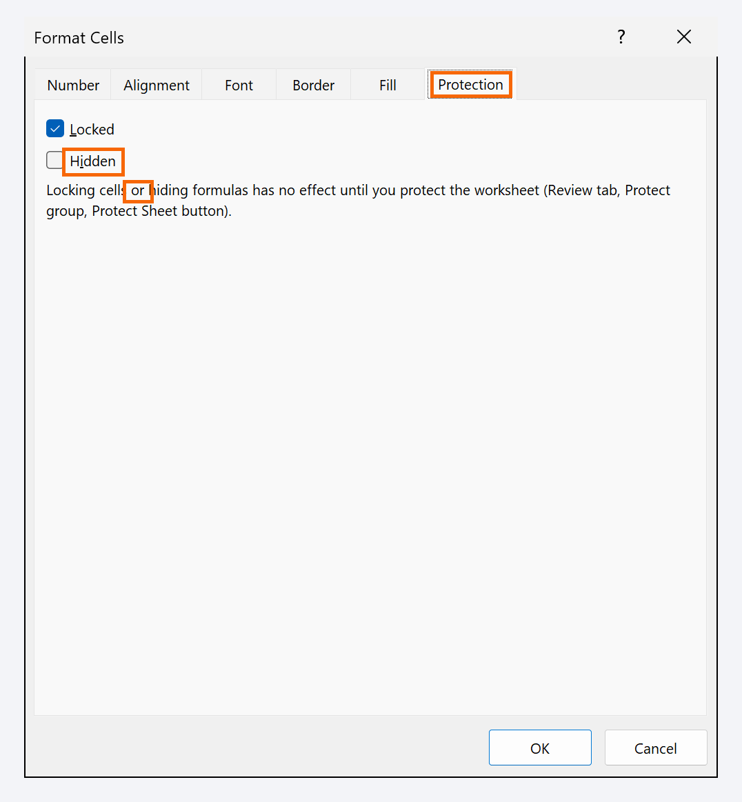
First, select C2:C11, press Ctrl+1 and, on the Protection tab, clear Locked: these will be the only editable cells. Then select the formulas in D2:D14, go back to Format Cells › Protection and check Hidden, so the formula bar doesn't reveal which cells they point to.
Finally, right-click the column E header › Hide. If it's a graded test, hide column D too: that way nobody sees their points while answering and can't keep trying letters until one sticks. If it's a practice quiz, leave D visible and it grades itself instantly.
Protect the sheet and give everyone their own copy
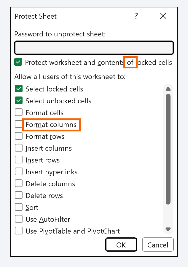
Go to Review › Protect Sheet. Clear Select locked cells (so people can only click the answers, and Tab jumps from one to the next) and leave Format columns unchecked, which is what stops anyone from unhiding the hidden columns. Add a password and click OK. All the details are in protect sheets and cells.
Save the file and send it as an attachment: each person gets their own copy, fills it in and sends it back. When it comes back, unprotect the sheet with your password and unhide the columns to see the grade.
Don't share a single OneDrive edit link with the whole class: everyone would type their answers into the same file, on top of the previous person's.
Expert tips
- Penalize wrong answers. If each wrong answer takes away a third of a point, as in many standardized tests, use
=MAX(0,ROUND((D13-(COUNTA(C2:C11)-D13)/3)*10/ROWS(E2:E11),1)).COUNTAcounts the answered questions; blanks aren't penalized. In the example: 7 right and 2 wrong give a 6.3. - Keep the key on another sheet. If you store the key on a sheet named Key, compare with
=IF(C2=Key!B2,1,0), hide that sheet (right-click the tab › Hide) and protect the workbook with Review › Protect Workbook so it can't be unhidden. - Letter grades. Add a letter next to the score:
=IF(D14>=9,"A",IF(D14>=8,"B",IF(D14>=7,"C",IF(D14>=6,"D","F")))). - Reuse the template. Save the empty quiz as a template and, for each new test, change only the questions and the key: validation, formulas and colors are already done.
Common mistakes and how to fix them
One question scores 0 for everyone even when the answer is right.
The key cell has an extra space or a different letter. Unprotect the sheet, unhide column E and type the letter on its own. You can also clean it with =TRIM(E2).
The grade shows as 6.66666667 or with lots of decimals.
ROUND is missing. Use =ROUND(D13*10/ROWS(E2:E11),1) to keep one decimal. Changing the number format only hides the decimals; it doesn't remove them.
Students see whether they're right as soon as they pick a letter and keep trying until they get it.
The points in column D are visible. Hide column D as well before protecting the sheet, or keep the color grading switched off with H1 set to No.
You protect the sheet and nobody can pick an answer.
You didn't unlock C2:C11. Unprotect the sheet, open Format Cells (Ctrl+1) › Protection, clear Locked for those cells and protect again.
In Excel for Mac the process is the same: Data › Data Validation for the list, Format Cells (⌘+1) › Protection for Locked and Hidden, and Review › Protect Sheet. The formulas don't change.
Frequently asked questions
Can someone see the key even though it's hidden?
Someone who knows Excel well, yes: protecting a sheet stops slips and curious clicks, but it isn't a security feature. For a high-stakes test, use a tool built for it, such as a Microsoft Forms quiz, which also grades itself and whose results you can open in Excel.
Can some questions be worth more than others?
Yes. Add a Weight column (for example in F2:F11) and change the point formula to =IF(C2=E2,F2,0). For the grade, divide by SUM(F2:F11) instead of ROWS(E2:E11).
Can I grade out of 100 instead of 10?
Yes. Multiply by 100 instead of 10: =ROUND(D13*100/ROWS(E2:E11),0). Seven right out of ten gives 70.
How do I see the whole class's grades together?
When the files come back, copy each person's grade into a summary sheet, or ask people to send back just the grade. If you run the quiz often with many people, a Microsoft Forms quiz collects every response in a single table.
Official sources
Microsoft documentation consulted for this guide.
Saved only in this browser.